Species detection probability#
Hint
Detection probability (aka detectability): The probability (likelihood) that an individual of the population of interest is included in the count at time or location i.
Detection probability categories are defined as follows:
Low:
- < 0.1 (Tobler & Powell, 2013)
- < 0.05 (Shannon et al., 2014)
- 0–0.37 (Chatterjee et al., 2021)Medium:
- 0.37–0.67 ()High:
- 0.67–1 (Chatterjee et al., 2021)
- /> 0.5 ()Unknown: Select this option if you’re not sure of the detection probability of your Target Species (single or multiple species)
Multiple: Select this option if your study include multiple Target Species.
Select “Unknown” if you’re not sure.
How this relates to study design
We use this information to adjust the recommended camera days per camera location and total number of camera days. For example, if the species is hard to detect, you may have to deploy cameras for longer to ensure you’ve sampled long enough to say that the species truly was not there (vs. it was there, but you did not detect it; “missed detections”, e.g., high cover of shrubs impeding your ability to see the species).
When you fail to detect an individual/species that was, in fact, present, this is called a “false absence”, which may lead to incorrect conclusions from the data. Understanding and correcting for sources of this type of error is often thought of in terms of probabilities (i.e., “detection probability” aka detectability).
Note! It’s not an exact science - Since detectability is affected by many other processes, it’s best incorporated in models (using your data) since this will result in the best suited information to inform your design.
How does that work?
Individuals and/or species are not always detected when they are present (i.e., detected “imperfectly”; MacKenzie et al., 2004). Missed detections occur or many reasons, including due characteristics of the environment (e.g., due to cover of vegetation), the time period (e.g., seasons), characteristics of the species (e.g., cryptic nature or small size), etc. The question here is asking about detection probability as it relates to the characteristics of the species (not the species in a particular habitat type or during a specific season).
You may need to consult previous studies to get a sense of which category is the most appropriate for your study and Target Species.
See also
Analysis aside
Many sources of detection error can be accounted for in analysis; this is done by assessing the relationships between the characteristics of the environment that we might expect to affect detection (e.g., cover of shrubs in front of the camera), and information on where (and when) the species was and was not detected. For example, there were consistently fewer detections on cameras placed in high shrub cover.
By assessing the relationships at locations repeatedly sampled over time, we begin to unravel the relationship between the environmental characteristics and missed detections on your cameras. We can then use this information to determine if we have sampled long enough (i.e., do we have enough information to differentiate between missed detections and true absences) and/or correct for this error in analysis by incorporating these effects in our models.
Before study design choices are made, there is one critical concept to understand in remote camera research, which may impact study design choices at all levels of the data hierarchy. Reliable use of remote cameras to detect wildlife species hinges on the assumption that what is captured on the cameras accurately reflects what is present on the landscape. However, species are often detected “imperfectly,” meaning that they are not always detected when they are present (i.e., imperfect detection; e.g., due to cover of vegetation, cryptic nature or small size) (MacKenzie et al., 2004). Imperfect detection can occur because the camera failed to capture an individual present at the site or because the animal was simply not present during the survey period (Martin et al., 2005).
Imperfect detection results in “false absences” and may lead to incorrect conclusions from the data. Understanding and correcting for sources of “false absences” is often thought of in terms of probabilities. Detection probability is the probability (likelihood) that an individual from the population of interest is included in the count at time or location i (MacKenzie & Kendall, 2002). Detection probability can be influenced through multiple processes and at multiple scales. Understanding the sources of “false absences” and factors that affect detection probabilities is an essential step when designing a study, deploying cameras and analyzing camera data.
The detection probability of an animal by a camera depends on three conditional probabilities (Pr) of detection that may operate alone or potentially in combination (Figure 1).
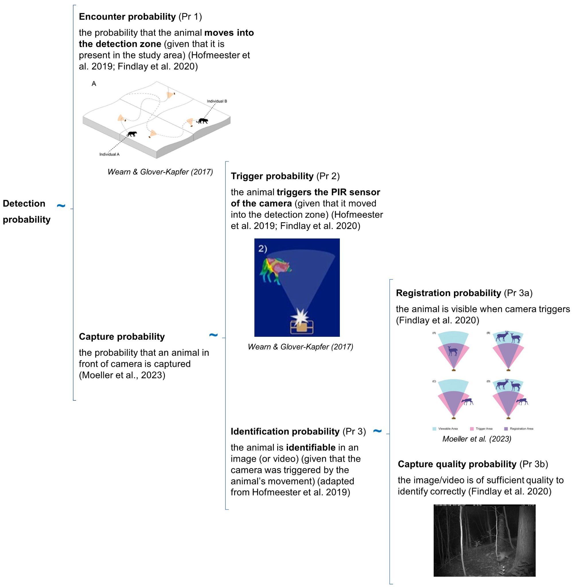
RCSC et al. (2024) - Fig. 1 Three conditional probabilities (Pr) of detection that may impact the detection probability of an animal (or species) by a camera (adapted from Moeller et al. [2023], Hofmeester et al. [2019], and Findlay et al. [2020]).
Detection probability can be affected by species-specific characteristics, Camera Model specifications and set-up, and environmental variables (Hofmeester et al., 2019). For example, species-specific characteristics (individuals or populations), such as body size (e.g., O’Brien et al., 2011), behaviour (e.g., Caravaggi et al., 2020; Rowcliffe et al., 2011), and rarity can influence detection probability, with larger, bolder and more common species generally having higher detection rates. ** Camera Model specifications and set-up**, such as the Trigger Sensitivity, Camera Height, or angle may affect detection probability in that smaller species might not be detected or identifiable if the Trigger Sensitivity is low, or the Camera Height or angle is too high. The Camera Direction could impact the probability of an animal triggering a camera if it is directed towards an object that impedes the or image quality (e.g. due to sun glare). Environmental factors (e.g., vegetation cover, snow depth) may affect detection probability and occurrence (e.g., Becker et al., 2022; Hofmeester et al., 2019; Iknayan et al., 2014; Steenweg et al., 2019). For example, a low number of detections in a densely vegetated site might be because of poor camera visibility or avoidance of this habitat by the species of interest.
Hofmeester et al. (2019) suggested there are six scales (orders) that may impact detection probability and that should be considered within an explicit time period (adapted from Hofmeester et al. [2019]; Figure 2):
Distribution range (1st order; i.e., the physical or geographical range of a species)
Landscape (2nd order; i.e., the location of an individual’s home range within the geographic range)
Habitat patch (3rd order; i.e., usage of habitat components within an individual’s home range)
Microsite (4th order; usage of microhabitats such as food items/feeding patches/nest sites/movement trails, etc. within a habitat)
Camera specification / set-up (5th order; i.e., factors that affect the probability that an animal triggers the camera if present)
Image (6th order; i.e., factors that affect correct identification of animals or individuals)
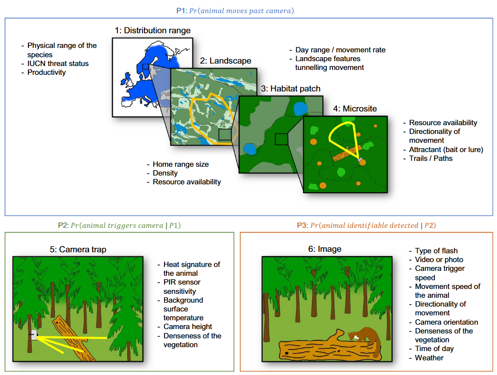
RCSC et al. (2024) – Fig. 2 Spatial scales (1-6) and processes that determine the detection probability (Hofmeester et al., 2019; abbreviated figure caption).
It is important to consider how all these factors and scales will impact study design. Unmeasured variation in detection probability can result in the inability to differentiate the effects of detection probability vs. habitat preference (Jennelle et al., 2002) and, in turn, cause erroneous estimates of occurrence and abundance (Burton et al., 2015; Dénes et al., 2015; Kays et al., 2021).
Factors that influence detection probability at the microsite and camera specification / set-up scales are likely to result in the largest biases and thus warrant the most consideration (see Hofmeester et al. [2019] for details). Therefore, it is particularly important to consider how to place cameras to avoid such biases. Deploying cameras in a consistent fashion (e.g., carefully ensuring that cameras are always set at the same Camera Height, orientation (), and angle is essential.
RCSC et al. (2024) - Fig. 1 Three conditional probabilities (Pr) of detection that may impact the detection probability of an animal (or species) by a camera (adapted from Moeller et al. [2023], Hofmeester et al. [2019], and Findlay et al. [2020]).
RCSC et al. (2024) - Fig. 2 Spatial scales (1-6) and processes that determine the detection probability (Hofmeester et al., 2019; abbreviated figure caption).
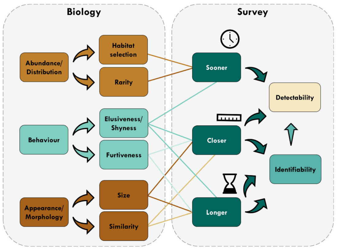
Tourani et al., (2020) - Fig. 1 Conceptual diagram showing different aspects of detectability during camera trap surveys and the modulating effect of biological characteristics. In addition to direct impacts on detectability, a longer visit and a closer image of focal species increase the chance of identifying the visitor, thereby increasing detectability. [Colour figure can be viewed at zslpublications.onlinelibrary.wiley.com].
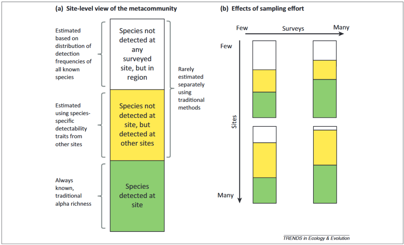
Iknayan et al., (2020) - Fig. 2 - Categories of species at surveyed sites resulting from imperfect detection and how they change with different temporal and spatial sampling strategies.
(A) The true (unknown) species pool of a metacommunity represented at a site comprises species that have been detected there (green bin), those that have not yet been detected at the site but have been detected at other surveyed sites (yellow bin), and those that have not yet been detected at this or any site but occur in the region (white bin). (B) As temporal and spatial replication (i.e., sampling effort) increases, knowledge of the species pool changes for both the site (green bins) and the metacommunity (green + yellow + white bins). When a site is surveyed few times, the relative size of each bin depends on the factors affecting detectability (Figure 1). If there are few sites and few surveys per site, a large portion of the metacommunity may not be detected (white bin of upper left rectangle), either at the site or at other sites. As the number of surveys per site increases (temporal replication) but not the number of sites surveyed (i.e., little spatial replication), the total number of species detected per site increases (green bin in upper right rectangle), mostly as a result of detecting species that are likely to occur at other sites (yellow bin). When the total number of sites surveyed increases (spatial replication) but not the number of surveys (i.e., little temporal replication), the number of species undetected in the region decreases (white bin in lower left rectangle), but the number of species detected per site remains the same (green bin). As both the number of surveys per site and the number of sites surveyed increase, a greater proportion of species in the metacommunity will be known (green + yellow bins in lower right rectangle), either from being directly detected at the site (green bin) or by being detected at other sites (yellow bin).
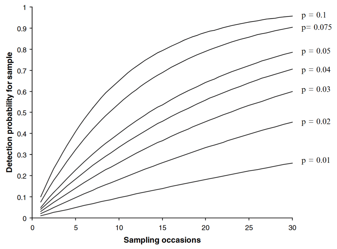
O’Connell et al. (2011) - Fig. 6.1 The cumulative likelihood of capturing an individual with a Pr(detection) per sampling occasion = p over K = 1 … 30 sampling occasions. As p and K increase, the likelihood of detection approaches 1.
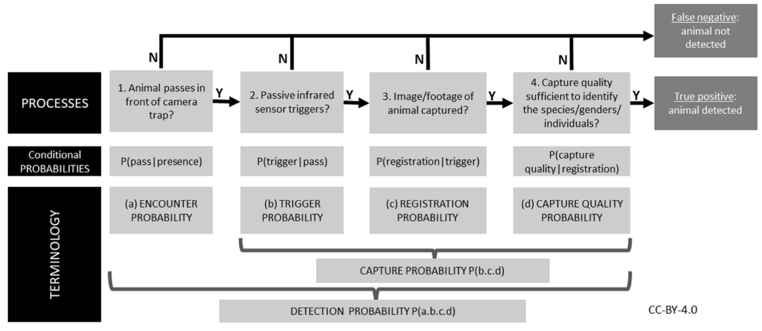
Findlay et al. (2020) - Fig. 1 The sequential processes required to detect an animal on a cameratrap given that it is present. Failure of any of these processes leads to a false-negative; therefore, detection success requires a positive outcome from all the component processes. Specific terminology we use in this study to quantify these processes is also shown. ‘Detection probability’ can thus be considered the product of a series of conditional probabilities representing each of these processes.
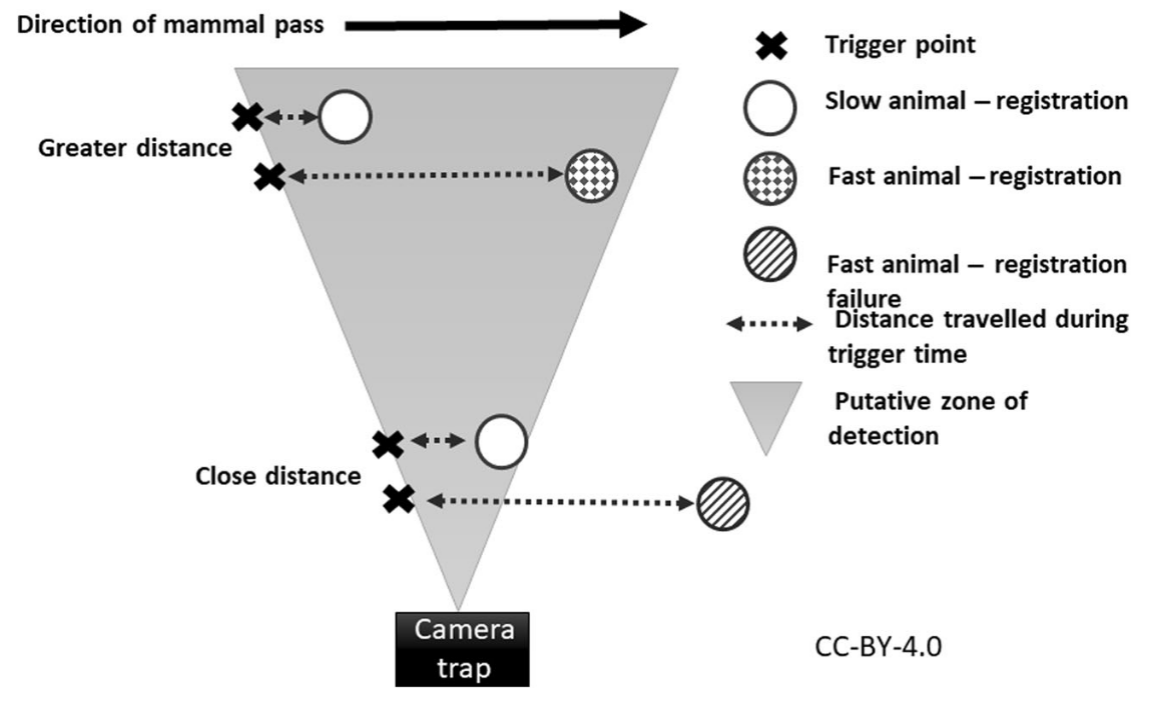
Findlay et al. (2020) - Fig. 8 Hypothesized mechanism showing how distance to camera-trap (CT) can interact with animal speed to influence registration probability. Registration probability is positively affected by distance due to the larger area within the field-of-view at greater distances. Conversely, faster moving animals can completely pass through the small width of the field-of view close to the CT before the camera takes an image
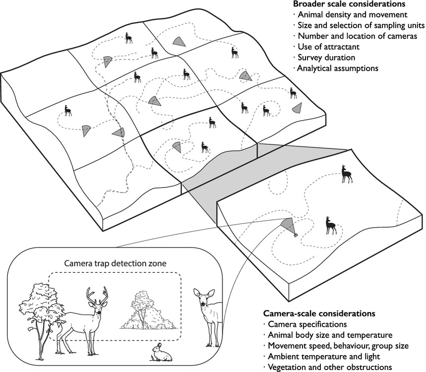
Burton et al. (2015) - Fig. 1 The detection of animals by camera traps is affected by ecological and observational processes occurring at both the local scale of the camera trap detection zone and the broader scale of the surrounding landscape. Explicitly accounting for these underlying processes is an important challenge for wildlife surveys with camera traps. (Image by Jeff Dixon).
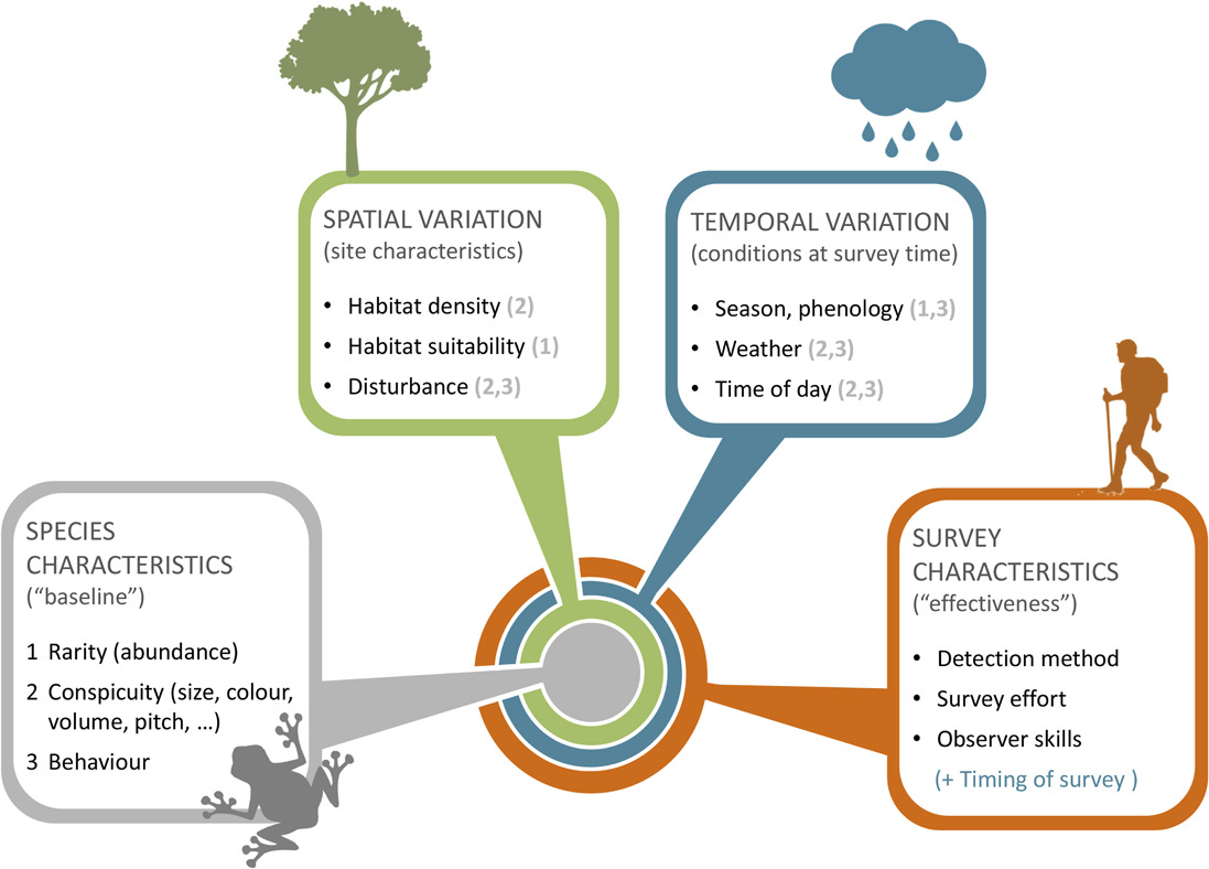
Guillera‐Arroita (2016) - Fig. 2 Factors determining species detectability. Whether a species tends to be more or less difficult to detect depends on a series of factors, described here with a nested structure.
At the core lie intrinsic characteristics of the species, including whether it is rare or abundant, its physical appearance (or vocal characteristics) and its behaviour. 2) These are modulated by site characteristics, potentially inducing spatial variation in species detectability. For instance, a given species may be more difficult to detect if the vegetation is denser at a site, if local abundance is lower due to the specific habitat type or if individuals are wary because the site experiences greater levels of disturbance than normal. Ambient noise (e.g. a road) can also make difficult aural detection of species at some sites. 3) Species detectability at a given site may also depend on factors that vary temporally. For instance, the species may display seasonal changes in behaviour or even abundance. Behaviour also normally changes with the time of day and weather conditions, and so do visibility (or audibility) conditions. 4) Finally, the detectability of a given species, at a given site and point in time, depends on the detection method used, the skills of the surveyor and the amount of survey effort (e.g. duration of a survey visit). In the diagram, the numbers in brackets indicate how factors that vary in space and time can modulate aspects defining a species ‘baseline’ detectability. This diagram highlights key factors affecting detectability and their interactions but it is not necessarily an exhaustive account. Differences in survey characteristics in space or time will induce spatial or temporal variation in detectability.
Probability of Detection: Eg 01
Probabilistic detection calculator (Mikkelä, 2024)
Online application used as an aid in sampling planning; calculates the probability of detecting disease (or other similar feature) with the given within-group prevalence and sample size for both finite and infinite group sizes. The detection means that at least one of the samples is detected positive. The sensitivity of the testing method can also be taken into account in the case of an imperfect test.
Additional information can be found here: https://zenodo.org/records/13120206
smsPOMDP (Pascal et al., 2020)
A Shiny r app to solve the problem of when to stop managing or surveying species under imperfect detection.
Additional information can be found here: conservation-decisions/smsPOMDP and https://besjournals.onlinelibrary.wiley.com/doi/full/10.1111/2041-210X.13501
Type |
Name |
Note |
URL |
Reference |
|---|---|---|---|---|
R package |
detect: analyzing wildlife data with detection error |
The R package implements models to analyze site occupancy and count data models with detection error. The package development was supported by the Alberta Biodiversity Monitoring Institute and the Boreal Avian Modelling (BAM) Project. |
Solymos, P., Moreno M., & Lele, S. R. (2024). detect: Analyzing Wildlife Data with Detection Error. R package version 0.5-0, https://github.com/psolymos/detect |
|
R Shiny app |
Probabilistic detection calculator (online application) |
Online application used as an aid in sampling planning; calculates the probability of detecting disease (or other similar feature) with the given within-group prevalence and sample size for both finite and infinite group sizes. |
Shiny app: https://detcal-shiny.2.rahtiapp.fi/; |
|
Related documents: https://zenodo.org/records/13120206 |
Mikkelä, A. (2024). Probabilistic detection calculator (online application). R shiny version v2. https://detcal-shiny.2.rahtiapp.fi/ |
|||