Species inventory#
Assumptions, Pros, Cons
No formal assumptions (Wearn & Glover-Kapfer, 2017)
Maximum flexibility for study design (e.g., camera days per camera location or use of lure (Rovero et al., 2013)) (Wearn & Glover-Kapfer, 2017)
Not reliable estimates for inference (‘considered as unfinished, working drafts’) (Wearn & Glover-Kapfer, 2017)
Species inventories are used to determine what species are present in an area during a given time period (Wearn & Glover-Kapfer, 2017). Inventories can be considered as a “checklist”, “minimum count”, or rapid assessment survey. The goal is to detect as many species as possible. With adequate sampling effort, species inventories may be help delineate species distribution, inform habitat associations, and provide an index of common species in an area. This assumes however that species can be reliably detected with sufficient effort, which may not be the case even for common or conspicuous species as many factors may influence species detection (e.g., sampling protocols, weather, observer experience etc.). Thus, only species presence (not absence) can be reliably determined. There are no attempts to quantify aspects of communities or populations, and no formal modeling approach are used.
Species accumulation curves can be used to determine if the survey effort is sufficient to estimate the number of species in an area. These curves plot the survey effort per unit time (x-axis) against the cumulative number of species detected (y-axis). The survey effort per unit time is the number of camera days (i.e., number of cameras multiplied by the number of days the cameras are operating) or survey days. The optimal survey effort occurs when the accumulation curve reaches an asymptote. This leveling of the curve indicates that very few, if any, new species are detected despite increasing survey effort. Refer to Species-accumulation curves for more information on species accumulation curves, and Tobler et al. (2008) for additional examples of species accumulation curves.
Various methods are available to assess the completeness of species inventories and to estimate the true species number in incomplete surveys (e.g., Colwell & Coddington, 1994; Colwell et al., 2004; Soberón & Llorente, 1993). These non-parametric and species richness estimators (Colwell & Coddington, 1994), with the former generally performing better in comparative studies (Walther & Moore, 2005).
Study design
The study design (e.g., camera arrangement) of species inventories is very flexible. However, if you’re targeting a single species the design should ideally still be informed by the species’ biology to maximize the likelihood of detecting individuals that are present. Information on preferred habitats, travel routes, or high activity areas (e.g., mineral licks, burrows) can be especially useful in determining where to strategically place cameras. When the species biology is well known, putting cameras at these targeted (non-random) locations may be beneficial. Alternatively, such as when the species biology is poorly known, randomly placing cameras across the study area may be the best approach to help ensures that all habitats are sampled in proportion to their availability (Wearn & Glover-Kapfer, 2017). The area sampled should in these cases be representative of the entire study area. Interestingly, in these cases, the area covered by cameras may have little effect on the number of species detected (Tobler et al., 2008).
Bait and Lure
The use of lure or bait may improve the likelihood of detecting some species (e.g., carnivores).
Camera Specifications
There are no specific guidelines for species inventories regarding camera features or deployment (e.g., number of cameras, camera days per location etc.). However, a camera model with a white flash, high sensitivity, large detection zone, and fast trigger speed may improve species detection (Rovero et al., 2013; Wearn & Glover-Kapfer, 2017).
Number of Cameras and Survey Duration
For species with a high probability of detection (e.g., small home range), deployment times can be short (e.g., 1-2 weeks) and moving cameras between locations can allow more sites to be sampled (Wearn & Glover-Kapfer, 2017). In contrast, cameras should be deployed longer in a location (e.g., 2-6 weeks; Wearn & Glover-Kapfer, 2017) for species with low probability of detection.
When the Target Species biology is poorly known, a general rule of thumb is to use a minimum of 20 single cameras per location within the study area, spaced 1-2 km apart, for ideally a minimum of 30 days per camera location and 1,000 overall camera days (Colyn et al., 2018; Rovero et al., 2013; Rovero & Tobler, 2010; Tobler et al., 2008; Wearn et al., 2013; Wearn & Glover-Kapfer, 2017). The more cameras deployed and/or locations sampled, generally the shorter the time needed to inventory an area. If fewer cameras are used, the cameras could be moved every 15 days, if feasible, to sample a larger area and avoid any biases associated with the camera locations (Rovero et al., 2013). In many areas, 1000-2000 camera days is sufficient to detect 60-70% of the species in the area (Ahumada et al., 2011; Tobler et al., 2008).
Analysis
Caution should be exercised in comparing the results of species inventories from different times of year within the same study area, or between study areas. The amount of sampling effort will need to be accounted for when examining any results.
Wearn & Glover-Kapfer (2017) – Fig. 7-3 Decision tree for short-term inventory work.
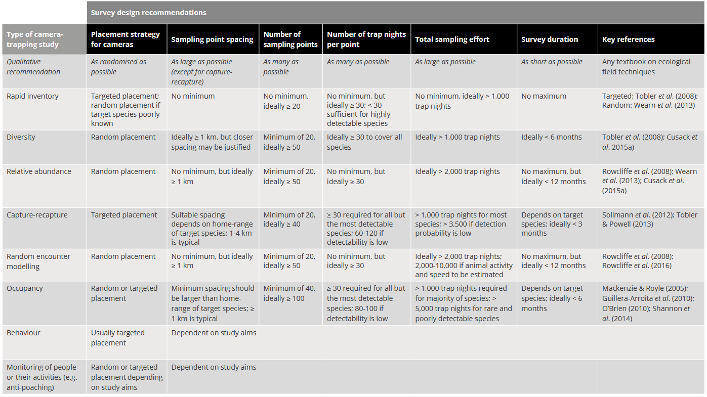
Wearn & Glover-Kapfer (2017) – Table 7.2 Recommended survey design characteristics for the major types of camera trap study, as taken from a broad review of the camera trap literature. Key references provide survey design advice or draw attention to important survey design considerations. The quantitative recommendations made here will often need to be adjusted to the specific context of a single study; this process can be informed by pilot studies or simulation work.

Check back in the future!
Type |
Name |
Note |
URL |
Reference |
|---|---|---|---|---|
Program |
Program “PRESENCE |
|||
This package allow users to simulate the required sample size for a desired level of precision in species richness. |
Software: <www.mbr-pwrc.usgs.gov/ software/presence.html>; |
Hines, J. E. (2006). PRESENCE - Software to estimate patch occupancy and related parameters. https://www.mbr-pwrc.usgs.gov/software/presence.html. |
||
Program |
GENPRES |
This package allow users to simulate the required sample size for a desired level of precision in species richness. |
||
Bailey, L. L., Hines, J. E., Nichols, J. D., & MacKenzie, D. I. (2007). Sampling Design Trade-Offs in Occupancy Studies with Imperfect Detection: Examples and Software. Ecological Applications, 17(1), 281-290. https://www.jstor.org/stable/40061993 |
||||
R function |
specaccum: Species Accumulation Curve |
The specaccum function finds species accumulation curves or the number of species for a certain number of sampled sites or individuals. |
Oksanen, J., Simpson, G. L., Blanchet, F. G., Kindt, R., Legendre, P., Minchin, P. R., O’Hara, R. B., Solymos, P., Stevens, M. H. H., Szoecs, E., Wagner, H., Barbour, M., Bedward, M., Bolker, B., Borcard, D., Carvalho, G., Chirico, M., De Caceres, M., Durand, S., … Weedon, J. (2024). vegan: Community Ecology Package. R package Version 2.6-6.1. <https://doi.org/10.32614/CRAN.package.vegan |
|
R package |
PresenceAbsence: An R package for presence absence analysis |
The PresenceAbsence package for R provides a set of functions useful when evaluating |
||
the results of presence-absence analysis. |
Freeman, E. A. & Moisen, G. (2008). PresenceAbsence: An R Package for Presence Absence Analysis. Journal of Statistical Software, 23(11). https://www.fs.usda.gov/rm/pubs_other/rmrs_2008_freeman_e001.pdf |
Ahumada, J. A., Silva, C. E. F., Gajapersad, K., Hallam, C., Hurtado, J., Martin, E., McWilliam, A., Mugerwa, B., O’Brien, T., Rovero, F., Sheil, D., Spironello, W. R., Winarni, N., & Andelman, S. J. (2011). Community Structure and Diversity of Tropical Forest Mammals: Data from a Global Camera Trap Network. Philosophical Transactions: Biological Sciences, 366(1578), 2703-2711. https://doi.org/10.1098/rstb.2011.0115
Colyn, R. B., Radloff, F., & O’Riain, M. J. (2018). Camera trapping mammals in the scrubland’s of the cape floristic kingdom - the importance of effort, spacing and trap placement. Biodiversity and Conservation, 27(2), 503-520. https://doi.org/10.1007/s10531-017-1448-z
Colwell, R. K., & Coddington, J. A. (1994).Estimating terrestrial biodiversity through extrapolation. Philosophical Transactions of the Royal Society of London. Series B, Biological Sciences, 345, 101-118. https://doi.org/10.1098/rstb.1994.0091
Colwell, R. K., Mao, C. X., & Chang, J. (2004). Interpolating, Extrapolating, and Comparing Incidence-based Species Accumulation Curves. Ecology, 85(10), 2717-2727. https://doi.org/10.1890/03-0557
Freeman, E. A. & Moisen, G. (2008). PresenceAbsence: An R Package for Presence Absence Analysis. Journal of Statistical Software, 23(11). https://www.fs.usda.gov/rm/pubs_other/rmrs_2008_freeman_e001.pdf
Alberta Remote Camera Steering Committee [RCSC], Stevenson, C., Hubbs, A., & Wildlife Cameras for Adaptive Management (WildCAM). (2024). Remote Camera Survey Guidelines: Guidelines for Western Canada. Version 3.0. Edmonton, Alberta. https://ab-rcsc.github.io/RCSC-WildCAM_Remote-Camera-Survey-Guidelines-and-Metadata-Standards/1_Survey-guidelines/1_0.1_Citation-and-Info.html
Rovero, F., Zimmermann, F., Berzi, D., & Meek, P. (2013). “Which camera trap type and how many do I need?” A review of camera features and study designs for a range of wildlife research applications. Hystrix, the Italian Journal of Mammalogy, 24(2), 148-156. https://doi.org/10.4404/hystrix-24.2-6316
Rovero, F., & Tobler, M., (2010). Camera trapping for inventorying terrestrial vertebrates. Manual on Field Recording Techniques and Protocols for All Taxa Biodiversity Inventories and Monitoring. https://www.researchgate.net/publication/229057405_Camera_trapping_for_inventorying_terrestrial_vertebrates
Soberón, J., & Llorente, J. (1993). The Use of Species Accumulation Functions for the Prediction of Species Richness. Conservation Biology, 7(3), 480-488. https://doi.org/10.1046/j.1523-1739.1993.07030480.x
Tobler, M. W., Pitman, R. L., Mares, R. & Powell, G. (2008). An Evaluation of Camera Traps for Inventorying Large- and Medium-Sized Terrestrial Rainforest Mammals. Animal Conservation, 11, 169-178. https://doi.org/10.1111/j.1469-1795.2008.00169.x
Walther, B. A., & Moore, J. L. (2005). The Concepts of Bias, Precision and Accuracy, and Their Use in Testing the Performance of Species Richness Estimators, with a Literature Review of Estimator Performance. Ecography, 28, 815-829. https://doi.org/10.1111/j.2005.0906-7590.04112.x
Wearn, O. R., Rowcliffe, J. M., Carbone, C., Bernard, H., & Ewers, R. M. (2013). Assessing the status of wild felids in a highly-disturbed commercial forest reserve in Borneo and the implications for camera trap Survey design. PLoS One, 8(11), e77598. https://doi.org/10.1371/journal.pone.0077598
Wearn, O. R., & Glover-Kapfer, P. (2017). Camera-Trapping for Conservation: A Guide to Best-ractices. WWF conservation technology series, 1, 1-181. http://dx.doi.org/10.13140/RG.2.2.23409.17767