Spatial capture-recapture (SCR) / Spatially explicit capture recapture (SECR)#
Assumptions, Pros, Cons
Demographic closure (i.e., no births or deaths) (Wearn & Glover-Kapfer, 2017)
Detection probability of different individuals is equal (Wearn & Glover-Kapfer, 2017)
or, for SECR, individuals have equal Detection probability at a given distance from the centre of their home range (Wearn & Glover-Kapfer, 2017)
Detections of different individuals are independent (Wearn & Glover-Kapfer, 2017)
Behaviour is unaffected by cameras and marking (Wearn & Glover-Kapfer, 2017)
Individuals do not lose marks (Wearn & Glover-Kapfer, 2017)
Individuals are not misidentified (Wearn & Glover-Kapfer, 2017)
Surveys are independent (Wearn & Glover-Kapfer, 2017)
For conventional models, geographic closure (i.e., no immigration or emigration) (Wearn & Glover-Kapfer, 2017)
Spatially explicit models have further assumptions about animal movement (Wearn & Glover-Kapfer, 2017; Rowcliffe et al., 2008; Royle et al., 2009; O’Brien et al., 2011); these include:
Home ranges are stable (Wearn & Glover-Kapfer, 2017)
Movement is unaffected by the cameras (Wearn & Glover-Kapfer, 2017)
Camera locations are randomly placed with respect to the distribution and orientation of home ranges (Wearn & Glover-Kapfer, 2017)
Distribution of home range centres follows a defined distribution (Poisson, or other, e.g., negative binomial) (Wearn & Glover-Kapfer, 2017)
Produces direct estimates of density or population size for explicit spatial regions (Chandler & Royle, 2013)
Allows researchers to mark a subset of the population / to take advantage of natural markings (Wearn & Glover-Kapfer, 2017)
Estimates are fully comparable across space, time, species and studies (Wearn & Glover-Kapfer, 2017)
density estimates obtained in a single model, fully incorporate spatial information of locations and individuals (Wearn & Glover-Kapfer, 2017)
Both likelihood-based and Bayesian versions of the model have been implemented in relatively easy-to-use software DENSITY and SPACECAP, respectively, as well as associated R packages) (Wearn & Glover-Kapfer, 2017)
Flexibility in study design (e.g., ‘holes’ in the trapping grid) (Wearn & Glover-Kapfer, 2017)
Open SECR (Efford, 2004; Borchers & Efford, 2008; Royle & Young, 2008; Royle et al., 2009) models exist that allow for estimation of recruitment and survival rates (Wearn & Glover-Kapfer, 2017)
Avoid ad-hoc definitions of study area and edge effects (Doran-Myers, 2018)
SECR (Efford, 2004; Borchers & Efford, 2008; Royle & Young, 2008; Royle et al., 2009) accounts for variation in individual Detection probability; can produce spatial variation in density; SECR (Efford, 2004; Borchers & Efford, 2008; Royle & Young, 2008; Royle et al., 2009) more sensitive to detect moderate-to-major populations changes (+/-20-80%) (Royle & Young, 2008; Royle et al., 2009)
Requires that individuals are identifiable (Wearn & Glover-Kapfer, 2017)
Requires that a minimum number of individuals are trapped (each recaptured multiple times ideally) (Wearn & Glover-Kapfer, 2017)
Requires that each individual is captured at a number of camera locations (Wearn & Glover-Kapfer, 2017)
Multiple cameras per station may be required to identify individuals; difficult to implement at large spatial scales as it requires a high density of cameras (Morin et al., 2022)
May not be precise enough for long-term monitoring (Green et al., 2020)
Cameras must be close enough that animals are detected at multiple camera locations (Wearn & Glover-Kapfer, 2017) (may be challenging to implement at large scales as many cameras are needed)’ (Chandler & Royle, 2013)
½ MMDM (Mean Maximum Distance Moved) will usually lead to an underestimation of home range size and thus overestimation of density (Parmenter et al., 2003; Noss et al., 2012; Wearn & Glover-Kapfer, 2017)
This section will be available soon! In the meantime, check out the information in the other tabs!
Note
This content was adapted from: The Density Handbook, “Using Camera Traps to Estimate Medium and Large Mammal Density: Comparison of Methods and Recommendations for Wildlife Managers” (Clarke et al., 2023)
Spatial capture-recapture (SCR) models can be applied to any survey method where animals are individually identifiable and trap locations are known: live trapping and tagging, DNA sampling, camera trapping, etc. (Royle et al., 2014). Here, we will discuss camera trap SCR.
SCR models break populations down into the activity, or home range, centres of individual animals. Let us first imagine we know the number and location of all individuals’ activity centres in a population. If we did, we could easily estimate density:
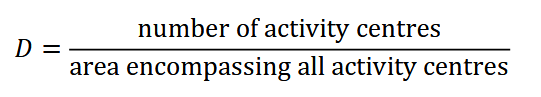
assuming each member of the population has an activity centre, and so the number of activity centres is equivalent to population size; and since the area encompassing all activity centres is the total area sampled by the camera array (i.e., the sampling frame; Sollmann, 2018). In reality, we do not know the number and location of activity centres – indeed, the estimated number and location of activity centres is the SCR model output.
To resolve the number and location of activity centres – and thus estimate density – SCR models combine information about 1) where animals are detected in space (using an observation model) and 2) how animals are distributed in space (using a spatial process model; Figure 4; Royle, 2016).
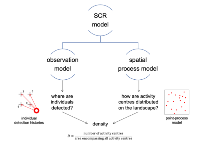
Clarke et al., 2023 - Fig. 4 SCR models are made up of two sub-models: an observation model, which describes where individual animals are detected (i.e., their detection histories); and a spatial process model, which describes how animals’ activity centres are distributed.
The observation model uses the record of where each individual was detected (i.e., individuals’ detection histories) to infer the location of each individual’s respective activity centre (Figure 5A; Chandler & Royle, 2013; Royle, 2016). It relies on the inverse relationship between detection probability and cameratrap-to-activity-centre distance: as the distance between a camera and an individual’s activity centre increases, the likelihood that individual will be detected there decreases (Figure 5B; Royle et al., 2014). So, animals will be detected most frequently at camera traps near their activity centres, and least frequently (or not at all) at camera traps far from their activity centres. Because the locations of activity centres are unknown, we use a spatial process model to approximate their distribution. Point-process models are a common choice (Royle, 2016). A point-process model is a random pattern of points in space (Baddeley, n.d.); it can be homogenous (completely spatially random) or inhomogeneous (the density of points depends on landscape/habitat covariates; (Royle, 2016).
Taken together: SCR essentially “downscales” density – a population-level estimator – to the level of the individual. The model asks: where does each animal live (Royle, 2016)? Although the location of animals’ activity centres is not known, we can use information about where individuals are captured (detection histories) and how activity centres are distributed in space (point-process model) to infer where they live, and thus estimate density (Royle, 2016). SCR can be implemented using many statistical frameworks, including full likelihood estimation (Borchers & Efford, 2008), dataaugmented maximum likelihood estimation (Royle et al., 2014), and data-augmented Bayesian estimation (Royle & Young, 2008; Morin et al., 2022).
When deploying cameras for SCR analysis, practitioners must balance the area covered by the camera array with trap spacing to maximize both the number of unique individuals captured and the number of spatial recaptures of each individual. A larger sampling area will yield a higher count of unique individuals; closely-spaced traps will yield a higher number of spatial recaptures (i.e., detections of the same individual at different camera traps; Royle et al., 2014). Both are important for SCR density estimation. Cameras should also be deployed across habitat types with different levels of use (Morin et al., 2022; Sun et al., 2014). Grid and clustered sampling designs can help meet all these needs (Clarke, 2019; Sun et al., 2014). Note that optimal camera trap placement and spacing will change with focal species, landscape and project limitations.
See Clark (2019), Dupont et al., (2021), Fleming et al., (2021), McFarlane et al., (2020), Nawaz et al., (2021), Romairone et al., 2018, Sollmann et al., (2012) and Sun et al., (2014) for more detailed explorations of SCR study design.
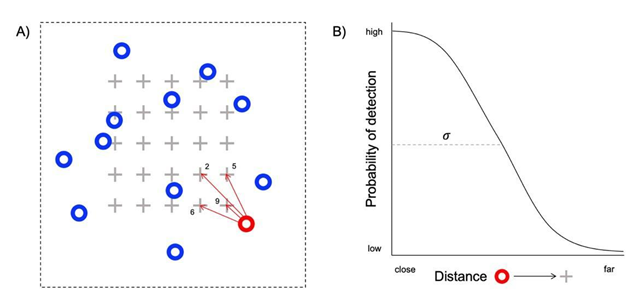
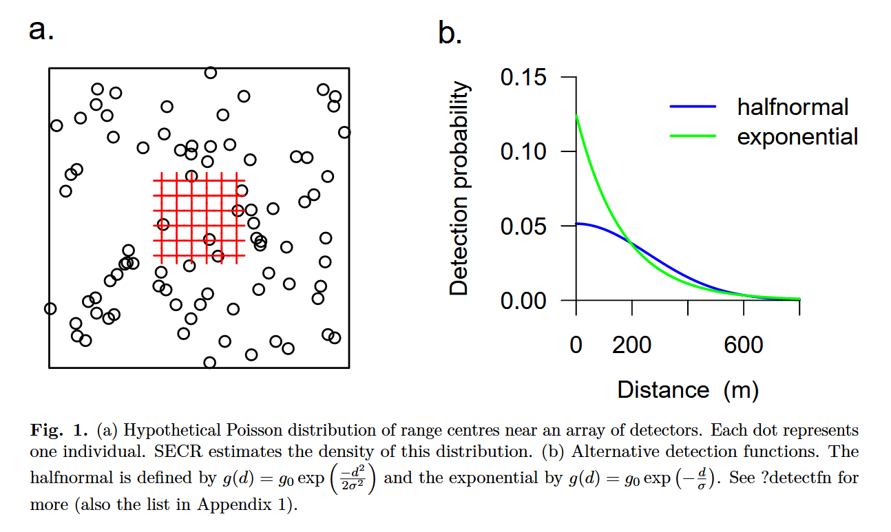
Clarke et al. (2023) – Fig. 5 Adapted from Morin et al., (2022) and Royle et al., (2014). A) A diagram of how the individual activity centres (circles) that make up a population might overlap with a camera array (grey crosses). The red circle highlights an example individual’s activity centre. The red arrows point towards camera stations where the red individual was detected; the numbers beside the camera stations show how many times the red individual was detected at each station. Note, the number and location of individual’s activity centres is not known, but rather inferred from the spatial pattern of detections (i.e., the number of detections of each individual at camera stations of known location). B) An example graph showing how the probability the red individual is detected at a camera station decreases with distance from its activity centre. This is reflected in A); as the distance between the red individual’s activity centre and a camera station increases, the number of detections dwindles. σ is the spatial scale parameter; it describes how detection probability decreases with increasing distance.
Another aspect of sampling design practitioners must consider is the number and configuration of cameras deployed at a station to identify animals to the individual. Left and right flanks may need to be photographed simultaneously, for example, to avoid assigning different identities to each side (Augustine et al., 2018); as another example, chest markings may need to be photographed from multiple angles at bait stations to be able to resolve identity (Proctor et al., 2022).
Clarke et al. (2023) – Fig. 4. SCR models are made up of two sub-models: an observation model, which describes where individual animals are detected (i.e., their detection histories); and a spatial process model, which describes how animals’ activity centres are distributed.
Clarke et al. (2023) - Fig. 5 Adapted from Morin et al., (2022) and Royle et al., (2014). A) A diagram of how the individual activity centres (circles) that make up a population might overlap with a camera array (grey crosses).
The red circle highlights an example individual’s activity centre. The red arrows point towards camera stations where the red individual was detected; the numbers beside the camera stations show how many times the red individual was detected at each station. Note, the number and location of individual’s activity centres is not known, but rather inferred from the spatial pattern of detections (i.e., the number of detections of each individual at camera stations of known location). B) An example graph showing how the probability the red individual is detected at a camera station decreases with distance from its activity centre. This is reflected in A); as the distance between the red individual’s activity centre and a camera station increases, the number of detections dwindles. σ is the spatial scale parameter; it describes how detection probability decreases with increasing distance.
University of Cape Town, 2024c - Slide 6 Observation process - The expected frequency of encountering an individual depends on the individual’s location in space.
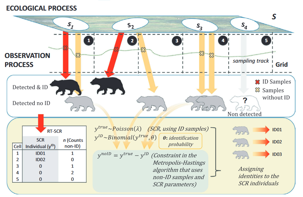
Jiménez et al. (2021) - Fig. 1 Graphical depiction of the random thinning spatial capture–recapture model. Random thinning SCR is hierarchical model with two processes: ecological (population size and location—si—of individuals) and observation.
In this model (like in standard SCR), the detection rate of each individual depends on (i) Euclidean distance between individual’s locations and traps (centroids of polygonal grid in the study case); (ii) baseline detection rate (λID) that here depends on sampling effort (length of transect in each polygon); and (iii) the scale parameter (σ) from the half-normal detection function, that describes the animal movement. In the observation process, we obtain two types of data: encounters with identification (yID) and non-ID data (ynoID) or counts. Random thinning SCR model uses ID data (in red) like in standard SCR to make inferences about population size and individuals’ distribution (including nonobserved individuals, in gray), but also uses the counts (in orange) with a constraint (ynoID = ytrue − yID) using a Metropolis–Hastings algorithm—in a mechanistic approach—to make a probabilistic reconstruction of the true encounter frequencies (ytrue), thus assigning identities to non-ID samples.


J. Andrew Royle, ’Spatial Capture-Recapture Modelling’
PAWS: Spatial Capture Recapture Data Analysis Part 1
PAWS: Spatial Capture Recapture Data Analysis Part 2
Introduction to Spatial Capture-Recapture with the oSCR Package
oSCR Package: Channel for the R package for the analysis of spatial encounter histories for inferences about spatial population ecology.
Efford, M. G., & Boulanger, J. (2019). Fast Evaluation of Study Designs for Spatially Explicit Capture-Recapture. Methods in Ecology and Evolution, 10(9), 1529-1535. https://doi.org/10.1111/2041-210X.13239
Type |
Name |
Note |
URL |
Reference |
|---|---|---|---|---|
Article |
Fast Evaluation of Study Designs for Spatially Explicit Capture–Recapture |
Efford, M. G., & Boulanger, J. (2019). Fast Evaluation of Study Designs for Spatially Explicit Capture-Recapture. Methods in Ecology and Evolution, 10(9), 1529-1535. https://doi.org/10.1111/2041-210X.13239 |
||
App/Program |
Program SPACECAP |
Note: this program is not longer available from cran (https://cran.r-project.org/web/packages/SPACECAP/index.html). |
Singh, P., Gopalaswamy, A. M., Royle, A. J., Kumar, N. S. & Karanth, K. U. (2010). SPACECAP: A Program to Estimate Animal Abundance and Density using Bayesian Spatially-Explicit Capture-Recapture Models. Wildlife Conservation Society - India Program, Centre for Wildlife Studies, Bangalure, India. Version 1.0. https://www.mbr-pwrc.usgs.gov/software/spacecap.html |
|
R package |
Package ‘secr’ |
Package info: https://CRAN.R-project.org/package=secr |
Efford, M. (2024a). Package ‘secr’: Spatially Explicit Capture-Recapture R package version 4.6.9. https://CRAN.R-project.org/package=secr; |
|
Youtube channel |
oSCR Package |
Multiple videos available related to the SCR approach; some may be useful even for those not using the oSCR package. |
oscrpackage206 (2020) oSCR Package. [Channel]. YouTube. https://www.youtube.com/channel/UCc87aAzhX7EUOalyCohzqsQ |
|
R package |
openCR: Open population capture-recapture models |
DENSITY | | https://CRAN.R-project.org/package=openCR | Efford, M. (2023). openCR: Open population capture-recapture models. R package version 2.2.6. https://CRAN.R-project.org/package=openCR |
| Powerpoint slides | SEEC Toolbox seminars - Spatial Capture-Recapture (SCR) models | ‘Greg Distiller provides a comprehensive introduction to SCR models and how to perform these in R’ | https://science.uct.ac.za/seec/stats-toolbox-seminars-spatial-and-species-distribution-toolboxes/spatial-capture-recapture-scr-modelling | University of Cape Town. (2024b). SEEC Toolbox seminars - Spatial Capture-Recapture (SCR) models. https://science.uct.ac.za/seec/stats-toolbox-seminars-spatial-and-species-distribution-toolboxes/spatial-capture-recapture-scr-modelling |
| R package | Package ‘oSCR’ | The ‘sim.SCR’ function
may be particularly useful. | Article: https://onlinelibrary.wiley.com/doi/10.1111/ecog.04551;
R package: jaroyle/oSCR | Sutherland, C., Royle, J. A., & Linden, D. W. (2019). oSCR: A spatial capture-recapture R package for inference about spatial ecological processes. Ecography, 42(9), 1459-1469. https://doi.org/10.1111/ecog.04551 |
| Tutorial | oSCR package [online resources] | This site contains tutorials; supplemental materials for the book Spatial Capture-Recapture by Royle, Chandler, Sollmann & Gardner (2013). | https://sites.google.com/site/spatialcapturerecapture/oscr-package/2-getting-started-with-oscr | Royle, J. Chandler, R. B., Sollmann, R., Gardner, B. (2013). Spatial capture-recapture. Academic Press, Waltham, MA, USA. 612 pp., ISBN: 978-0-12-405939-9. https://pubs.usgs.gov/publication/70048654 |
| App/ProgramR package | DENSITY | Software for analysing capture-recapture data from passive detector arrays. | https://doi.org/10.32800/abc.2004.27.021 | Efford, M. G., Dawson, D. K., & Robbins, C. S. (2004). DENSITY: Software for analysing capture-recapture data from passive detector arrays. Animal Biodiversity and Conservation, 27(1), 217-228. https://doi.org/10.32800/abc.2004.27.0217 |
| resource10_type |
Augustine, B. C., Royle, J. A., Kelly, M. J., Satter, C. B., Alonso, R. S., Boydston, E. E., & Crooks, K. R. (2018). Spatial Capture-Recapture with Partial Identity: An Application to Camera Traps. The Annals of Applied Statistics, 12(1), 67-95. https://doi.org/10.1214/17AOAS1091
Baddeley, A. (N.D.) Spatial Point Processes and Their Applications. School of Mathematics & Statistics, University of Western Australia. https://www.researchgate.net/profile/Mohamed-Mourad-Lafifi/post/One-dimensional-spatial-point-processes/attachment/59d641b279197b807799d9fb/AS%3A436024913469445%401480967848679/download/07-baddeley-point-process-poisson-coverage-sensor-simulation.pdf
Borchers, D. L., & Efford, M. G. (2008). Spatially Explicit Maximum Likelihood Methods for Capture-Recapture Studies. Biometrics, 64(2), 377-385. https://doi.org/10.1111/j.1541-0420.2007.00927.x
Chandler, R. B., & Royle, J. A. (2013). Spatially explicit models for inference about Density in unmarked or partially marked populations. The Annals of Applied Statistics, 7(2), 936-954. https://doi.org/10.1214/12-aoas610
Clarke, J. D. (2019).comparing Clustered Sampling Designs for Spatially Explicit Estimation of Population Density. Population Ecology, 61, 93-101. https://doi.org/10.1002/1438-390X.1011
Clarke, J., Bohm, H., Burton, C., Constantinou, A. (2023). Using Camera Traps to Estimate Medium and Large Mammal Density: Comparison of Methods and Recommendations for Wildlife Managers. https://doi.org/10.13140/RG.2.2.18364.72320
Dupont, G., Royle, J. A., Nawaz, M. A., & Sutherland, C. (2021). Optimal sampling design for spatial capture-recapture. Ecology, 102(3), e03262. https://doi.org/10.1002/ecy.3262
Efford, M. G., Dawson, D. K., & Robbins, C. S. (2004). DENSITY: Software for analysing capture-recapture data from passive detector arrays. Animal Biodiversity and Conservation, 27(1), 217-228. https://doi.org/10.32800/abc.2004.27.0217
Efford, M. G., & Boulanger, J. (2019). Fast Evaluation of Study Designs for Spatially Explicit Capture-Recapture. Methods in Ecology and Evolution, 10(9), 1529-1535. https://doi.org/10.1111/2041-210X.13239
Efford, M. (2023). openCR: Open population capture-recapture models. R package version 2.2.6. https://CRAN.R-project.org/package=openCR
Efford, M. (2024a). Package ‘secr’: Spatially Explicit Capture-Recapture R package version 4.6.9. https://CRAN.R-project.org/package=secr
Efford, M. (2024b). secr 4.6 - spatially explicit capture-recapture in R. https://cran.r-project.org/web/packages/secr/vignettes/secr-overview.pdf
Fleming, J., Grant, E. H. C., Sterrett, S. C., & Sutherland, C. (2021). Experimental evaluation of spatial capture-recapture study design. Ecological Applications, 31(7), e02419. https://doi.org/10.1002/eap.2419
Gopalaswamy, A. M., Royle, J. A., Hines, J. E., Singh, P., Jathanna, D., Kumar, N. S., & Karanth, K. U. (2012). Program SPACECAP: software for estimating animal Density using spatially explicit capture-recapture models. Methods in Ecology and Evolution, 3(6), 1067-1072. https://doi.org/10.1111/j.2041-210X.2012.00241.x
Proctor, M. F., Garshelis, D. L., Thatte, P., Steinmetz, R., Crudge, B., McLellan, B. N., McShea, W. J., Ngoprasert, D., Nawaz, M. A., Te Wong, S., Sharma, S., Fuller, A. K., Dharaiya, N., Pigeon, K. E., Fredriksson, G., Wang, D., Li, S., & Hwang, M. (2022). Review of field methods for monitoring Asian bears. Global Ecology and Conservation, 35, e02080. https://doi.org/10.1016/j.gecco.2022.e02080
McFarlane, S., Manseau, M., Steenweg, R., Hervieux, D., Hegel, T., Slater, S., & Wilson, P. J. (2020). An assessment of sampling designs using SCR analyses to estimate abundance of boreal caribou. Ecology and Evolution, 10(20), 11631-11642. https://doi.org/10.1002/ece3.6797
Morin, D. J., Boulanger, J., Bischof, R., Lee, D. C., Ngoprasert, D., Fuller, A. K., McLellan, B., Steinmetz, R., Sharma, S., Garshelis, D., Gopalaswamy, A., Nawaz, M. A., & Karanth, U. (2022).comparison of methods for estimating Density and population trends for low-Density Asian bears. Global Ecology and Conservation, 35, e02058 https://doi.org/10.1016/j.gecco.2022.e02058
Nawaz, M. A., Khan, B. U., Mahmood, A., Younas, M., Din, J. U., & Sutherland, C. (2021). An empirical demonstration of the effect of study design on density estimations. Scientific Reports, 11(1), 13104. PubMed-not-MEDLINE. https://doi.org/10.1038/s41598-021-92361-2
oscrpackage206 (2020) oSCR Package. [Channel]. YouTube. https://www.youtube.com/channel/UCc87aAzhX7EUOalyCohzqsQ
Sollmann, R., Gardner, B., & Belant, J. L. (2012). How does Spatial Study Design Influence Density Estimates from Spatial capture-recapture models? PLoS One, 7, e34575. https://doi.org/10.1371/journal.pone.0034575
Sun, C. C., Fuller, A. K., & Royle., J. A. (2014). Trap Configuration and Spacing Influences Parameter Estimates in Spatial Capture-Recapture Models. PLoS One, 9(2): e88025. https://doi.org/10.1371/journal.pone.0088025
Romairone, J., Jiménez, J., Luque-Larena, J. J., & Mougeot, F. (2018). Spatial capture-recapture design and modelling for the study of small mammals. PLOS ONE, 13(6), e0198766. https://doi.org/10.1371/journal.pone.0198766
Royle, J. A., Converse, S. J., & Freckleton, R. (2014). Hierarchical spatial capture-recapture models: modelling population Density in stratified populations. Methods in Ecology and Evolution, 5(1), 37-43. https://doi.org/10.1111/2041-210x.12135
Royle, A. J. (2016, Oct 17). ‘Spatial Capture-Recapture Modelling.’ CompSustNet [Video]. YouTube. https://www.youtube.com/watch?v=4HKFimATq9E
Royle, A. J. (2020, Oct 26) Introduction to Spatial Capture-Recapture. oSCR Package, [Video]. YouTube. https://www.youtube.com/watch?v=yRRDi07FtPg
Royle, J. A., & Young, K. V. (2008). A hierarchical model for spatial capture-recapture data. Ecology, 89(8), 2281-2289. https://doi.org/10.1890/07-0601.1
University of Cape Town. (2024a). SEEC Toolbox seminars https://science.uct.ac.za/seec/stats-toolbox-seminars
University of Cape Town. (2024b). SEEC Toolbox seminars - Spatial Capture-Recapture (SCR) models. https://science.uct.ac.za/seec/stats-toolbox-seminars-spatial-and-species-distribution-toolboxes/spatial-capture-recapture-scr-modelling