Spatial count (SC) model / Unmarked spatial capture-recapture#
Assumptions, Pros, Cons
Camera locations are close enough together that animals are detected at multiple cameras (Chandler & Royle, 2013; Clarke et al., 2023)
Demographic closure (i.e., no births or deaths) (Chandler & Royle, 2013; Clarke et al., 2023)
Geographic closure (i.e., no immigration or emigration) (Chandler & Royle, 2013; Clarke et al., 2023)
Detections are independent (Chandler & Royle, 2013; Clarke et al., 2023)
Animals’ activity centres are randomly dispersed (Chandler & Royle, 2013; Clarke et al., 2023)
Animals’ activity centres are stationary (Chandler & Royle, 2013; Clarke et al., 2023)
Does not require individual identification (Clarke et al., 2023)
Produces imprecise estimates even under ideal circumstances unless supplemented with auxiliary data (e.g., telemetry) (Doran-Myers, 2018; Chandler & Royle, 2013; Sollmann et al., 2013a; Sollmann et al., 2013b)
Precision decreases with an increasing number of individuals detected at a camera’ (Morin et al., 2022) (as overlap of individuals’ home ranges increases) (Augustine et al., 2019; Clarke et al., 2023)
Not appropriate for low density or elusive species when recaptures too few to confidently infer the number and location of activity centres’ (Clarke et al., 2023; Burgar et al., 2018)
Not appropriate for high-density populations with evenly spaced activity centres (camera[-specific] counts will be too similar and impair activity centre inference)’ (Clarke et al., 2023)
Ill-suited to populations that exhibit group-travelling behaviour’ (Sun et al., 2022; Clarke et al., 2023)
Study design (camera arrangement) can dramatically affect the accuracy and precision of density estimates’ (Clarke et al., 2023; (Undefined, 2018))
Cameras must be close enough that animals are detected at multiple camera locations (may be challenging at large scales as many cameras are needed)’ (Chandler & Royle, 2013; Clarke et al., 2023)
This section will be available soon! In the meantime, check out the information in the other tabs!
Note
This content was adapted from: The Density Handbook, “Using Camera Traps to Estimate Medium and Large Mammal Density: Comparison of Methods and Recommendations for Wildlife Managers” (Clarke et al., 2023)
A spatial count (SC) model is essentially a spatial capture-recapture (SCR; see Spatial capture-recapture (SCR) / Spatially explicit capture recapture (SECR)) model with an extension to account for unmarked animals’ unknown identities (Royle et al., 2014). SC, then, is formulated in much the same way as SCR: populations are treated as collections of individual activity (or home range) centres, and spatial detection data is used to infer the number and locations of these activity centres (see Spatial capture-recapture (SCR) / Spatially explicit capture recapture (SECR)). Instead of identifying animals and constructing individual detection histories (i.e., each individual’s spatial pattern of detections), however, SC uses trap-specific counts (i.e., the tally of animal detections at each trap of known location) and the correlation structure among trapspecific counts to estimate the number and location of activity centres (Royle et al., 2014, Sun et al., 2022).
Like SCR, an SC model is composed of a spatial process model and an observation model. The spatial process model, which describes how activity centres are distributed across the landscape, is a homogeneous point-process model – a completely random pattern of points in space (Baddeley, no date; Royle, 2016). The observation model, which describes where individuals are detected on the landscape, is constructed as if we know each individual’s detection history and the size of the population (Chandler & Royle, 2013). As Royle et al. (2014) put it: “[SC] is formulated in terms of the data we wish we had, i.e., the typical [detection] history data observed in [SCR] studies of marked animals.” We can construct an SC model in this way because trap-specific counts of animals arise from those animals’ detection histories; in other words, counts are a simplified version of the data that would have been collected, had individuals been identifiable (Chandler & Royle, 2013, Sun et al., 2022).
To relate trap-specific counts to detection histories, we use the equation:
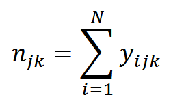
where n𝑗𝑘 is the count of animals at sampling location 𝑗 and during sampling period 𝑘; 𝑁 is population size; and 𝑦𝑖𝑗𝑘 is individual 𝑖’s detection history at sampling location 𝑗 and during sampling period 𝑘 (Royle et al., 2014). So, the trap- and period-specific count n𝑗𝑘 – the information we gather for SC – is the same as the sum of every individual’s encounter history at that trap – the information we gather for SCR (Royle et al., 2014).
To approximate population size, we take a data augmentation approach. Population size 𝑁 is treated as a subset of some larger, hypothetical population of size 𝑀 (the “augmented” population; Royle & Dorazio, 2012), such that:
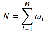
where 𝑀 ≫ 𝑁 and 𝜔𝑖 is the probability of existence of individual 𝑖 within population 𝑁 (Chandler & Royle, 2013, Sun et al., 2022). 𝜔𝑖 is Bernoulli distributed – an animal can be present (i.e., 𝜔𝑖 = 1) or absent (i.e., 𝜔𝑖 = 0) – and depends on the number of detections at traps and the distance between traps and individuals’ activity centres (Chandler & Royle, 2013, Sun et al., 2022).
Note that, for SC, a “trap” is simply a tool or method for collecting count data. Trap types include hair snags, track plates, acoustic recording devices, human point-count observers and camera traps (Chandler & Royle, 2013, Royle et al., 2014). We will refer to camera traps for the remainder of this section.
The aim of SC sampling design is to infer the number and location of activity centres by inducing correlation (i.e., linear relation) between the number and location of detections (Burgar et al., 2019, Chandler & Royle, 2013, Sollmann et al., 2018, Sun et al., 2022). To this end, camera traps must be deployed close enough together that individuals will be detected at multiple locations (Chandler & Royle, 2013). Grid or clustered designs may be best (Burgar et al., 2019, Clarke, 2019, Sun et al., 2014).
Simulations and Field Experiments
The relatively few studies that have tested SC models suggest that they tend to produce fairly accurate but imprecise density estimates.
A study on fishers showed that, compared to genetic SCR, SC underestimated density and estimates were less precise (Burgar et al., 2018).
Evans and Rittenhouse (2018) found that SC yielded accurate but less precise estimates of black bear density than camera trap SCR.
Another study compared estimates of caribou density from SC with estimates from the spatial partial identity model (SPIM; see and Spatial Partial Identity Model (2-flank SPIM))). In this system, SC likely underestimated density compared with SPIM – perhaps because the model interpreted captures of many individuals as recaptures of a few individuals – and was less precise and more variable year-toyear (Sun et al., 2022).
SC was used to estimate the densities of caribou, moose, wolf, coyote and black bear populations in the oil sands region of Alberta (Burgar et al., 2019). Estimates for all species were imprecise; some had confidence intervals with upper and lower bounds that differed more than 10-fold. The authors note, however, that other density estimation methods used in the region (e.g., aerial surveys) are not more precise than SC (Burgar et al., 2019). The researchers also simulated their data, finding that SC tended to underestimate density when the number of captures and spatial recaptures (i.e., spatially-correlated detections between cameras) were low.
Box 1. The unmarked models that follow estimate density within the collective viewshed area (i.e., the combined fields-of-view of all cameras in a network) and assume that this estimate applies to the larger study area (Gilbert et al., 2020). This is in contrast to spatial capture-recapture (SCR; see Spatial capture-recapture (SCR) / Spatially explicit capture recapture (SECR)) models and derivatives – including spatial count (SC; see Spatial count), spatial mark-resight (SMR; see Spatial mark-resight and the spatial partial identity model (SPIM; see and Spatial Partial Identity Model (2-flank SPIM)) – which estimate density over a defined area.
Check back in the future!
Type |
Name |
Note |
URL |
Reference |
|---|---|---|---|---|
R package |
‘nimble’ package |
Burgar, J. M., Stewart, F. E. C., Volpe, J. P., Fisher, J. T., & Burton, A. C. (2018). Estimating Density for species conservation: comparing camera trap spatial count models to genetic spatial capture-recapture models. Global Ecology and Conservation, 15, Article e00411. https://doi.org/10.1016/j.gecco.2018.e00411
Burgar, J. M., Burton, A. C., & Fisher, J. T. (2019). The importance of considering multiple interacting species for conservation of species at risk. Conservation Biology, 33(3), 709-715. https://doi.org/10.1111/cobi.13233
Chandler, R. B., & Royle, J. A. (2013). Spatially explicit models for inference about Density in unmarked or partially marked populations. The Annals of Applied Statistics, 7(2), 936-954. https://doi.org/10.1214/12-aoas610
Clarke, J. D. (2019).comparing Clustered Sampling Designs for Spatially Explicit Estimation of Population Density. Population Ecology, 61, 93-101. https://doi.org/10.1002/1438-390X.1011
Clarke, J., Bohm, H., Burton, C., Constantinou, A. (2023). Using Camera Traps to Estimate Medium and Large Mammal Density: Comparison of Methods and Recommendations for Wildlife Managers. https://doi.org/10.13140/RG.2.2.18364.72320
Evans, M. J. & Rittenhouse, T. A. G. (2018). Evaluating Spatially Explicit Density Estimates of Unmarked Wildlife Detected by Remote Cameras. The Journal of Applied Ecology 55(6), 2565-74. https://doi.org/10.1111/1365-2664.13194
Gilbert, N. A., Clare, J. D. J., Stenglein, J. L., & Zuckerberg, B. (2020). Abundance Estimation of Unmarked Animals based on Camera-Trap Data. Conservation Biology, 35(1), 88-100. https://doi.org/10.1111/cobi.13517
Royle, A. J. (2016, Oct 17). ‘Spatial Capture-Recapture Modelling.’ CompSustNet [Video]. YouTube. https://www.youtube.com/watch?v=4HKFimATq9E
Royle, J. A., & Dorazio, R. M. (2012). Parameter-expanded data augmentation for Bayesian analysis of capture-recapture models. Journal of Ornithology, 152(S2), 521-537. https://doi.org/10.1007/s10336-010-0619-4
Royle, J. A., Converse, S. J., & Freckleton, R. (2014). Hierarchical spatial capture-recapture models: modelling population Density in stratified populations. Methods in Ecology and Evolution, 5(1), 37-43. https://doi.org/10.1111/2041-210x.12135
Sun, C. C., Fuller, A. K., & Royle., J. A. (2014). Trap Configuration and Spacing Influences Parameter Estimates in Spatial Capture-Recapture Models. PLoS One, 9(2): e88025. https://doi.org/10.1371/journal.pone.0088025
Sun, C., Burgar, J. M., Fisher, J. T., & Burton, A. C. (2022). A Cautionary Tale Comparing Spatial Count and Partial Identity Models for Estimating Densities of Threatened and Unmarked Populations. Global Ecology and Conservation, 38, e02268. https://doi.org/10.1016/j.gecco.2022.e02268
Sollmann, R. (2018). A gentle introduction to camera‐trap data analysis. African Journal of Ecology, 56, 740-749. https://doi.org/10.1111/aje.12557
Gilbert, N. A., Clare, J. D. J., Stenglein, J. L., & Zuckerberg, B. (2020). Abundance Estimation of Unmarked Animals based on Camera-Trap Data. Conservation Biology, 35(1), 88-100. https://doi.org/10.1111/cobi.13517