Instantaneous sampling (IS)#
See also
Assumptions, Pros, Cons
Demographic closure (i.e., no births or deaths) (Moeller et al., 2018)
Geographic closure (i.e., no immigration or emigration) (Moeller et al., 2018)
Detection is perfect (detection probability ‘p’ = 1) (Moeller et al., 2018)
Can be efficient for estimating abundance of common species (with a lot of images) (Moeller et al., 2018)
Flexible assumption of animals’ distribution (Moeller et al., 2018)
Requires accurate counts of animals (Moeller et al., 2018)
Detection is perfect (detection probability ‘p’ = 1) (Moeller et al., 2018)
Reduced precision (Moeller et al., 2018)
This section will be available soon! In the meantime, check out the information in the other tabs!

Note
This content was adapted from: The Density Handbook, “Using Camera Traps to Estimate Medium and Large Mammal Density: Comparison of Methods and Recommendations for Wildlife Managers” (Clarke et al., 2023)
The instantaneous sampling model (IS) is an extension of the space-to-event model (STE; see Space-to-event (STE)) that uses counts of animals in time-lapse images – instead of the area until an animal is first detected – to estimate density (Moeller et al., 2018). As with the STE, all cameras in a randomly-deployed array are programmed to take time-lapse images at predefined intervals (e.g., every hour) to get instantaneous “snapshot” samples of the study area. During image processing, the number of animals in each photograph is recorded. Thus, the IS is essentially a series of fixed-area point counts (Moeller et al., 2018): camera traps act as “standing observers” tabulating the number of individuals seen within a set area and time.
The IS equation is as follows:
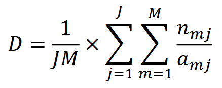
where 𝐽 is the total number of sampling occasions, 𝑀 is the total number of camera stations, and 𝑛𝑚𝑗 is the count of animals in the viewshed and 𝑎𝑚𝑗 is the area of the viewshed at station 𝑚 on sampling occasion 𝑗 (Moeller et al., 2018).
Simulations and Field Experiments
The IS is relatively untested opposite its sister models. Simulations have shown that the IS is unbiased to animal movement speed or population size, so is applicable to slow- and fast-moving animals and to low- and high-density populations (Moeller et al., 2018). When tested on a population of elk in Idaho, the IS produced a similar density estimate as an aerial survey, but which was less precise than both TTE- and STE-derived estimates (Moeller et al., 2018).
Moeller & Lukacs (2021) The spaceNtime workflow for count data. The user will go through five major steps for STE, TTE, and IS analyses. If the user has presence/absence (0 and 1) data instead of count data, the IS analysis is not appropriate, and the IS pathway should be removed from the flowchart.
Check back in the future!
Type |
Name |
Note |
URL |
Reference |
|---|---|---|---|---|
R package |
spaceNtime: an R package for estimating abundance of unmarked animals using camera-trap photographs |
free and open-source R package designed to assist in the implementation of the STE and TTE models, along with the IS estimator |
<annam21/spaceNtime |
Clarke, J., Bohm, H., Burton, C., Constantinou, A. (2023). Using Camera Traps to Estimate Medium and Large Mammal Density: Comparison of Methods and Recommendations for Wildlife Managers. https://doi.org/10.13140/RG.2.2.18364.72320
Moeller, A. K., Lukacs, P. M., & Horne, J. S. (2018). Three Novel Methods to Estimate Abundance of Unmarked Animals using Remote Cameras. Ecosphere, 9(8), Article e02331. https://doi.org/10.1002/ecs2.2331