Relative abundance indices#
Assumptions, Pros, Cons
Many assumptions exist (since used for many approaches) (Wearn & Glover-Kapfer, 2017)
Simple to calculate and technically possible (even with small sample sizes when robust methods might fail) (Wearn & Glover-Kapfer, 2017)
Relative abundance indices often do correlate with abundance (Wearn & Glover-Kapfer, 2017)
Calibration with independent density estimates is possible (Wearn & Glover-Kapfer, 2017)
Difficult to draw inferences (a large number of assumptions); comparisons across space, time, species, and studies are difficult (Wearn & Glover-Kapfer, 2017)
Requires stringent study design (e.g., random sampling, standardized methods) (Wearn & Glover-Kapfer, 2017)
Detection rates from cameras cannot be used as an index to compare relative abundance across species (Rowcliffe & Carbone, 2008)
This section will be available soon! In the meantime, check out the information in the other tabs!

Note
This content was adapted from: The Density Handbook, “Using Camera Traps to Estimate Medium and Large Mammal Density: Comparison of Methods and Recommendations for Wildlife Managers” (Clarke et al., 2023)
In ecology, relative abundance (RA) is any count of animals or animal sign (e.g., number of deer sighted, number of bird vocalizations per unit time, number of moose tracks per kilometer of transect) that is assumed to correlate with absolute abundance (O’Brien, 2011). RA is a controversial index for two reasons: 1) there is often no documented relationship between the number of animals or signs observed and population size (i.e., index validation), and 2) detection probability is assumed to be constant between the areas, times or species being compared (O’Brien, 2011; Thompson et al., 1998).
To the first point: the relationship between the number of animals or signs and abundance is rarely established (Burton et al., 2015). Researchers often assume that counts and population size scale linearly – but many other kinds of relationships are possible. When the assumed relationship between counts and abundance diverges from the actual relationship, inferences from RA are not very meaningful (Thompson et al., 1998). Validating a count-abundance relationship requires comparison with a robust, accurate estimate of absolute density (e.g., Krebs et al., 1987; Rovero & Marshall, 2009; Villette et al., 2016).
To the second point: consider the canonical equation,
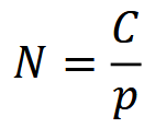
where 𝑁 is population size, 𝐶 is the count of animals or signs and 𝑝 is detection probability (Anderson, 2001; Brennan, 2019). This equation underlies many estimators of abundance, including capture-recapture (CR; see Capture-recapture (CR) / Capture-mark-recapture (CMR)) and distance sampling (DS; see Distance sampling) methods (O’Brien, 2011). RA comparisons assume that detection probability 𝑝 is constant across space, time or species, and can therefore be ignored (Anderson, 2001; O’Brien, 2011; Sollmann et al., 2013b), such that:
so count essentially becomes a surrogate for population size.
Assuming constant detection probability 𝑝 is problematic, since the likelihood an animal or sign is counted during a survey will vary with observational, environmental, and habitat- and species-specific factors, which in turn can vary with time (Anderson, 2001). For example: at site A, animals may be difficult to spot in dense vegetation, while at site B, animals may be easy to spot in open grassland; and the effects of vegetation on observability may differ seasonally. If the effects of vegetation on detectability are not accounted for, how can we be sure that differences in animal counts at site A and B are due to true differences in abundance, and not simply artefacts of detection bias (Sollmann et al., 2013b)?
In a camera trapping context, RA is the comparison of detection rates across space, time or species – where detection rates are typically reported as the number of images per 100 trap days, but can also be reported in terms of the total number of detections, other units of effort (e.g., camera trap hours), proportion of stations with detections, etc. (Burton et al., 2015). As with other kinds of RA surveys, comparisons of camera trap detection rates can confound abundance with animal behaviour and observability (Anderson, 2001; Burton et al., 2015).
RA has been criticized as an abundance estimator. Anderson (2001) condemned the index as “unprofessional,” while O’Brien (2011) called it a “metric of last resort.” Sollmann et al. (2013b) used simulations to determine that camera trap RA analyses did not detect changes in big cat density, and called use of the index for wildlife management “alarming.” Nevertheless, some researchers have had success with the method and/or have argued for its conceptual and practical advantages (e.g., Rowcliffe & Carbone, 2008; Johnson, 1980; Palmer et al., 2018; Rovero & Marshall, 2009). Broadley et al. (2019) used simulations to show that RA could be sensitive to density-dependent movement, but generally tracked abundance well. Banks-Leite (2014) emphasized the importance of careful sampling design and protocols to control for variation in detectability, arguing that researchers should not solely rely on statistical corrections.
Ultimately, there is no “silver bullet” and researchers must carefully consider their inferential objectives and potential sources of sampling and estimation bias when choosing response variables and modelling frameworks for camera trap data.
Modified from Gilbert et al. (2020) - Fig 3.
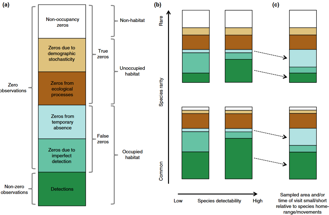
Dénes et al. (2015) - Fig. 1. Mechanisms that cause different types of zero observations in count surveys and how species rarity, detectability and sampling effort affect them.
(a) False zeroes are due to either imperfect detection or temporary absence. True zeroes can occur when the sample unit is unoccupied by the species, due to demographic stochasticity or due to ecological mechanisms such as unsuitable habitat or interspecific competition. (b) For common and detectable species (lower right), the majority of zeroes can be expected to result from ecological processes. As species detectability decreases, new false zeroes arise due to detection error (lower left). Species rarity results in fewer detections (dark green bars), additional true zeroes arise from unoccupied sample units (white bars) and increased demographic stochasticity (beige bars). (c) When the area sampled and/or the time of visit are small/ short relative to the species home range or movements, individuals may not be available for detection during the survey, resulting in additional false zeroes and fewer non-zero observations.
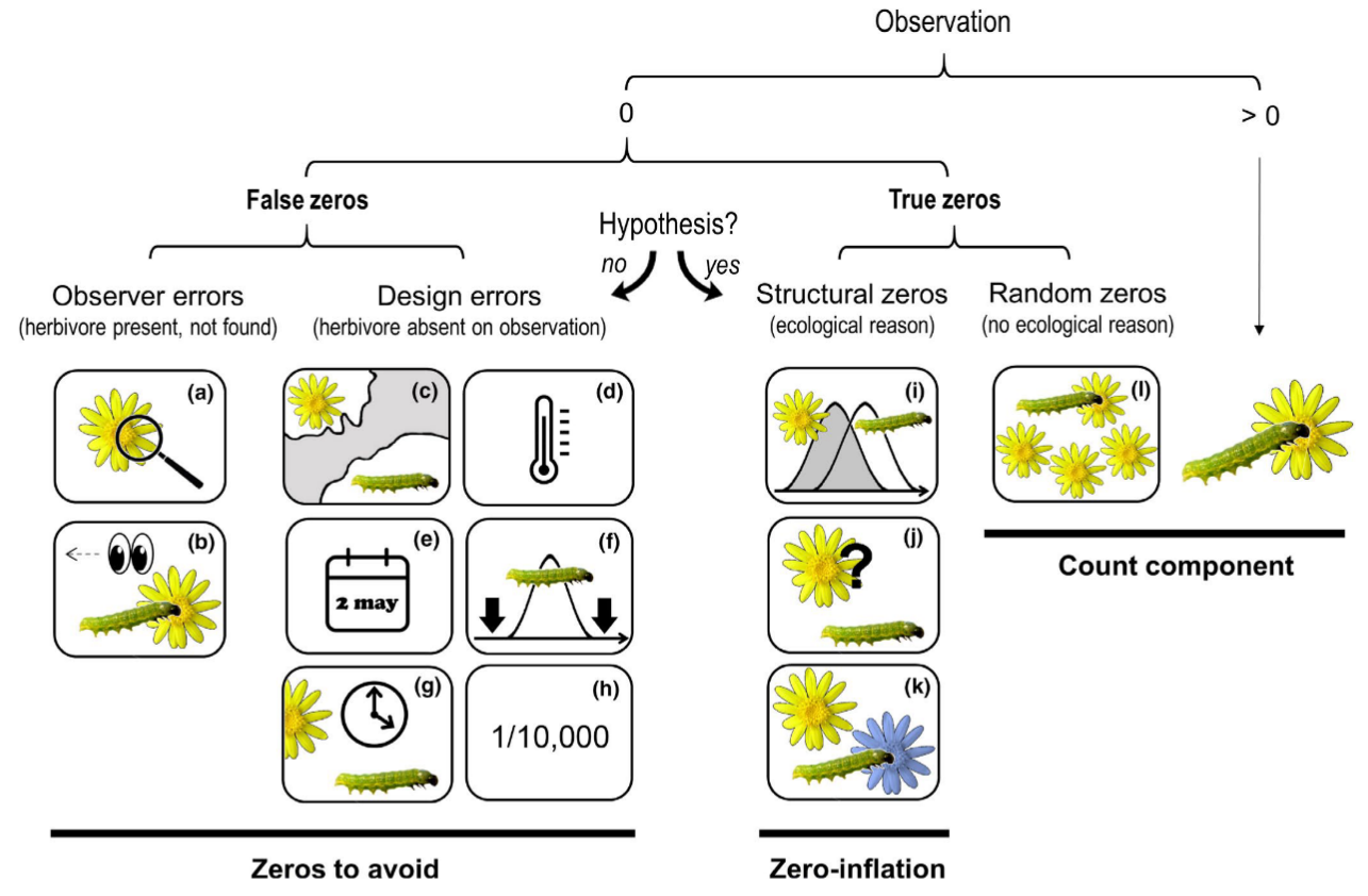
Blasco-Moreno et al. (2019) - Fig 1. Different sources of zeros that could emerge in count data.
The example shows the presence (>0) or absence (0) of herbivores on a plant species. Zeros due to the lack of experience of the observer (a–b) or resulting from a poor experimental design (c–h) are called False Zeros and should be minimized when performing the experiment. Structural Zeros, that is, zeros related to the ecological system under study (i–k), and Random Zeros emerging from the sampling variability (l) are known as True Zeros. Classifying a zero as a design error or structural zero depends on whether the event is part of the hypotheses tested. Only when the study includes the possibility of a zero value as part of the hypotheses (e.g. the study aims to test whether the interaction is occurring) the resulting zeros would be structural and should be included in the statistical analysis. The following text explains different scenarios that would result in a zero value, and, in brackets, how errors due to false zeros can be minimized: (a) the insects or the damage exerted are so small that the observer cannot detect them [sample when the insects are expected to be well developed]; (b) the observer does not see the herbivore (e.g. it is mistaken for a seed) or the damage is associated to other causes not related to herbivory (e.g. mechanical damage during sampling, pathogens, etc.) [the observer should be trained properly]; (c) the distributional areas of herbivores and plants are not coincident [know the species distribution before sampling]; (d) a herbivore is not present in a certain location within its distributional area, for example due to the microclimatic conditions [sample in habitats with adequate environmental conditions for a herbivore, or perform replicate surveys in different areas]; (e) a single survey is conducted, and is not coincident with the herbivore phenology [know the herbivore life cycle or perform long‐term surveys]; (f) a long‐term survey is conducted, but the low sampling frequency does not enable capture of the presence of the herbivore [sample on a more frequent basis]; (g) herbivores are not found because they are absent at the time of sampling [record plant damage instead of the presence of insects]; (h) herbivores are so infrequent that the design cannot capture their presence [perform extensive sampling with a high number of replicates]; (i) phenology of plants and herbivores are not completely coincident at a temporal level; (j) herbivores do not recognize a plant as a potential host; (k) herbivores recognize a plant as a host but prefer to feed on another species and (l) the herbivore population is not large enough to saturate the available plant resources.
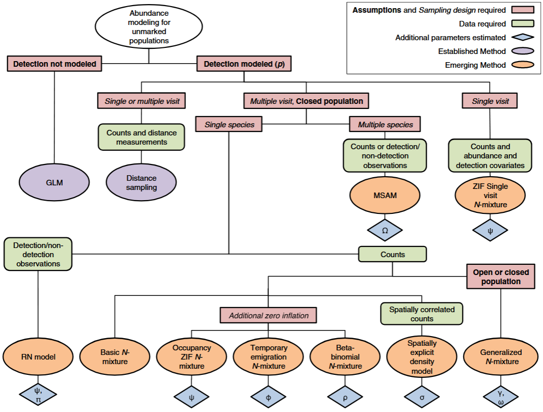
** Denes et al. (2015) - Fig. 2** Summary of the main modelling approaches for estimating abundance of unmarked animal populations described in the text.
Red boxes represent important model assumptions (in bold) and sampling design requirements (in italic), green boxes represent the types of input data used by each model, lilac and orange ellipses represent established and emerging methods, respectively, and blue diamonds represent additional parameters estimated. w indicates models that estimate potential occupancy probability, / indicates models that estimate probability of temporary emigration from the sample unit, and q indicates models that account for correlation in detection of individuals. p is site-level detection probability, c and x are arrival rate and survival probability parameters, respectively, r is the spatial correlation in counts, and Ω is the probability that a species is present in the supercommunity.
Using Hurdle Models to Analyze Zero-Inflated Count Data
Hurdle models
Zero-inflated Poisson (ZIP) regression
Poisson Regression Review
Poisson Regression: Zero Inflation (Excessive Zeros)
Fitting Poisson and zero-inflated Poisson models.
A Shiny app allows you to visualize data by using R scripts without having to interact with the R script itself. This Shiny app will allow you to plot your Relative Abundance microbiome data in an easy-to-view format. If this is your first time utilizing this Shiny app, follow the step below to start visualising your data now!
Type |
Name |
Note |
URL |
Reference |
|---|---|---|---|---|
R resource |
abmi.camera.extras: Animal Density from Camera Data > Probabilistic gaps |
Main resource page: https://mabecker89.github.io/abmi.camera.extras/index.html; |
Becker, M. Huggard, D. J., & Alberta Biodiversity Monitoring Institute [ABMI]. (2020). abmi.camera.extras. R package version 0.0.1. https://mabecker89.github.io/abmi.camera.extras |
|
App/Program |
Introduction to Camera Trap Data Management and Analysis in R > Chapter 12 Activity |
https://bookdown.org/c_w_beirne/wildCo-Data-Analysis/activity.html |
WildCo Lab (2021d). Chapter 12 Activity. https://bookdown.org/c_w_beirne/wildCo-Data-Analysis/activity.html |
|
App/Program |
R package “activity” |
Provides functions to express clock time data relative to anchor points (typically solar); fit kernel density functions to animal activity time data; plot activity distributions; quantify overall levels of activity; statistically compare activity metrics through bootstrapping; evaluate variation in linear variables with time (or other circular variables). |
Rowcliffe, M. (2023). Package ‘activity. R package version 1.3.4. https://cran.r-project.org/web/packages/activity/index.html |
|
R package |
R package “overlap” |
Estimates of Coefficient of Overlapping for Animal Activity Patterns |
Campbell, A. (2024). Package ‘overlap’. R package version 0.3.9. https://cran.r-project.org/web/packages/overlap/index.html |
|
Tutorial |
Chapter 6 Modeling Relative Abundance |
https://cornelllabofornithology.github.io/ebird-best-practices/abundance.html |
Strimas-Mackey, M., Hochachka, W. M., Ruiz-Gutierrez, V., Robinson, O. J., Miller, E. T., Auer, T., Kelling, S., Fink, D., & Johnston, A. (2023). Best Practices for Using eBird Data. Version 2.0. https://ebird.github.io/ebird-best-practices. Cornell Lab of Ornithology, Ithaca, New York. |
|
R package |
glmmTMB: Generalized Linear Mixed Models using Template Model Builder |
Brooks, M., Bolker, B., Kristensen, K., Maechler, M., Magnusson, A., Skaug, H., Nielsen, A., Berg, C., & Van Bentham, K. (2017). glmmTMB: Generalized Linear Mixed Models using Template Model Builder. R package version 1.1.10. https://doi.org/10.32614/CRAN.package.glmmTMB |
||
R package |
R package “zicounts” |
Counts data models: zero-inflation as well as interval icensored |
||
R package |
R package “DHARMa” |
Can be used to assess goodness-of-fit of a mixed effect model via quantile–quantile (Q–Q) plots of standardized residuals |
Hartig, F. (2019). DHARMa: Residual Diagnostics for Hierarchical (Multi-Level/Mixed) Regression Models. R package version 0.2.2, https://CRAN.R-project.org/package=DHARMa |
|
R package |
R package “Pscl” |
Jackman, (2024). R package ’Pscl’. R package version 1.5.9. https://cran.r-project.org/web/packages/pscl/index.html |
||
R package |
R package “countreg” |
Can be used to assess goodness-of-fit of a mixed effect hurdle model via rootograms (Kleiber & Zeileis, 2016) |
||
https://rdrr.io/rforge/countreg/f/inst/doc/countreg.pdf> |
Zeileis, A., Kleiber, C., & Jackman, S. (2008). Regression Models for Count Data in R. Journal of Statistical Software, 27(8). https://doi.org/10.18637/jss.v027.i08 |
A guide to modeling outcomes that have lots of zeros with Bayesian hurdle lognormal and hurdle Gaussian regression models |
https://www.andrewheiss.com/blog/2022/05/09/hurdle-lognormal-gaussian-brms |
+check others