Distance sampling (DS)#
Assumptions, Pros, Cons
Random or systematic random placements (consistent with the assumption that points are placed independently of animal locations) (Howe et al., 2017)
Camera locations are randomly placed relative to animal movement (Palencia et al., 2021)
Detection is perfect (detection probability ‘p’ = 1) at focal area */ distance 0 (Palencia et al., 2021)
Demographic closure (i.e., no births or deaths) and geographic closure (i.e., no immigration or emigration) (animal density is constant during the survey) (Palencia et al., 2021)
Animal movement and behaviour are unaffected by the cameras (Palencia et al., 2021)
Animals are detected at initial locations (e.g., they do not change course in response to the camera prior to detection) (Palencia et al., 2021)
Distances are measured exactly (however if the data from different distances will be grouped (‘binned’) for analysis later, an accuracy of +*/- 1m may suffice) (Palencia et al., 2021)
Snapshot moments selected independently of animal locations (Palencia et al., 2021)
A shortcut to controlling for variation in detection distances by only counting individuals within a short distance with an unobstructed view, and well sampled across cameras and species (Wearn & Glover-Kapfer, 2017)
density estimates are unbiased by animal movement ‘since camera-animal distance is measured at a certain instant in time (intervals of duration t apart)’ (Howe et al., 2017; Clarke et al., 2023)
Can be applied to low-density populations (Howe et al., 2017; Clarke et al., 2023)
Does not require individual identification (Howe et al., 2017)
May require discarding a portion of the dataset (when the best fitting model truncates the dataset) (Wearn & Glover-Kapfer, 2017)
Biased by movement speed (Palencia et al., 2021)
Best suited to larger animals; the smaller the focal species, the lower remote cameras must be set, which reduces the depth of the viewshed, and thus sampling size and the flexibility of the model’ (Howe et al., 2017; Clarke et al., 2023).
Does not permit inference about spatial variation in abundance (unless using hierarchical distance which can model spatial variation as a function of covariates) (Gilbert et al., 2020; Clarke et al., 2023)
Calculating camera-animal distances can be labour-intensive and time-consuming (however, recently developed techniques (e.g., Johanns et al., 2022) show promise for simplifying and automating the process) (Clarke et al., 2023)
Requires a good understanding of the focal populations’ activity patterns; density estimates can be biased (e.g., under-estimated) when regular periods of inactivity are not accounted for (using detection times to infer periods of activity may help overcome this limitation)’ (Howe et al., 2017; Palencia et al., 2021; Clarke et al., 2023)
Tends to underestimate density (Howe et al., 2017; Twining et al., 2022; Clarke et al., 2023)
{{ mod_ds_con_08 }
This section will be available soon! In the meantime, check out the information in the other tabs!
Note
This content was adapted from: The Density Handbook, “Using Camera Traps to Estimate Medium and Large Mammal Density: Comparison of Methods and Recommendations for Wildlife Managers” (Clarke et al., 2023)
Distance sampling (DS) theory was developed in the early 1990s to estimate density from line- or point-transect surveys, including aerial surveys (e.g.,
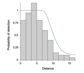
Clarke et al. (2023) - Fig. 6 An example detection function. The probability of detecting an animal decreases with increasing distance from the observer.
The DS model was adapted for use with camera trap data by Howe et al. (2017). Camera trap DS capitalizes on the similarities between camera trap surveys and human-observer point transect surveys – for example, both cameras and people tabulate the number of animals seen in a “snapshot” moment from a point in space (Buckland, 2006). There are, however, important differences to account for. For one: in human-observer studies, a point is sampled for an instant, and only one or a few times total; a camera, in contrast, samples the same point for a long period of time (Palencia et al., 2021). For another: human observers can pivot 360º around a point to count animals, while cameras are fixed in place and sample only a fraction of a circle (Howe et al., 2017). Camera trap DS must therefore include inputs of time and viewshed angle. The equation derived by Howe et al. (2017) is:
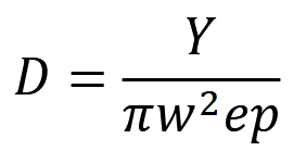
where 𝑌 is the number of detection events, 𝑤 is the truncation distance (i.e., the distance beyond which animal-camera distances are no longer considered), 𝑒 is the sampling effort, and 𝑝 is the probability of capturing an image of an animal within distance 𝑤 (Howe et al., 2017).
To calculate sampling effort 𝑒: let us first consider temporal effort. At a given camera, temporal effort is a function of the camera’s total sampling time 𝐻 and a predetermined interval 𝑡 units of time apart, at which the distance between camera and animal(s) is measured, such that temporal effort at the camera is 𝐻/𝑡 (Howe et al., 2017). If that same camera has a viewshed angle of 𝜃 radians, the fraction of a circle it samples is 𝜃 / 2π.
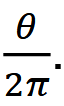
Taken together, sampling effort can therefore be expressed as:
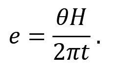
To estimate the probability of capturing an animal 𝑝: practitioners must estimate the horizontal distance 𝑟 between a camera and the centre of every animal detected, at each snapshot moment 𝑡 intervals apart, for as long as animals are within the viewshed (Howe et al., 2017). Howe et al. (2017) recommend a 𝑡 of 0.25 to 3 seconds; if the focal species is fast-moving or rare, and/or cameras have fast trigger speeds, practitioners should use a smaller 𝑡. Measurements of 𝑟 can then be inputted into a detection function, 𝑓(𝑟), which describes the probability an animal at distance 𝑟 is detected given 0 ≤ 𝑟 ≤ 𝑤 – producing an estimate of 𝑝 (Buckland et al., 2015).
Options for measuring camera-animal distance 𝑟 include: 1) comparing images of animals to reference images of field crew or objects at known distances from the camera (manually or automated; Haucke et al., 2022, Howe et al., 2017); 2) placing permanent reference objects at known distances from the camera so they are visible in every capture (Palencia et al., 2021); 3) physically measuring out camera-animal distances in the field, using animal images as references (Rowcliffe et al., 2011); and 4) a recently-developed, fully-automated approach (PJcs/DistanceEstimationTracking) which does not require reference images or objects (Johanns et al., 2022).
If the species of interest is regularly and predictably inactive (e.g., rests at night), estimates of density must be corrected for activity level to minimize bias (Howe et al., 2017; Palencia et al., 2021). Practitioners may choose to set total sampling time 𝐻 as the time the study population was active and available for detection; another option is to correct density 𝐷** for the proportion of time animals are active, such that:
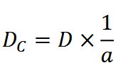
where 𝐷𝐶 is the corrected density estimate and 𝑎 is activity level (Howe et al., 2017; Palencia et al., 2021). Activity level is determined as per Rowcliffe et al. (2014).
Simulations & Field Experiments
Howe et al. (2017) ran simulations of “complex” animal movement patterns (i.e., animals moved with variable speeds, meandered, and rested periodically), and found that, when periods of rest were excluded from analyses, the DS model produced unbiased and precise estimates of density (CV / 0.10). When periods of rest were included, in contrast, DS performed poorly and inconsistently – whether animals rested within the viewshed or outside of the viewshed (i.e., were not detected). Animal activity patterns should therefore be considered when implementing the DS model; practitioners should have a strong understanding of when their species of interest is active versus inactive. Note that population and camera trap densities were both quite high in this simulation – 10 animals/km2 and 6.25 camera traps/km2 (Howe et al., 2017).
In northwestern Africa, camera trap DS produced higher estimates of duiker density than line-transect surveys – a method generally thought to underestimate the densities of forest-dwelling ungulates (Howe et al., 2017). The researchers collected video data.
Another study in northwestern Africa found that the DS model performed variably for different species (Cappelle et al., 2021). DS density estimates of a common ungulate – duiker – were comparable to previous estimates (line-transect surveys and Howe et al.’s (2017) camera trap DS study), and similarly precise. For semi-arboreal chimpanzees, DS-derived density estimates were biased low and depended greatly on measures of activity level (i.e., the proportion of the day chimpanzees were on the ground and available for detection). Compared with other studies:
DS performed inferiorly to spatial capture-recapture (SCR; see section Spatial capture-recapture (SCR) / Spatially explicit capture recapture (SECR)) with individual identification (Després‐Einspenner et al., 2017, Cappelle et al., 2019).
DS estimates were, however, comparable to labour-intensive line-transect nest surveys. The DS model performed inconsistently for rare species in this system, producing reasonable estimates of leopard density but questionable estimates of elephant density.
DS-derived leopard density was similar to a previous study combining collar, camera and track data (Cappelle et al., 2021, Jenny, 1996). DS-derived elephant density was nearly double that from previous line-transect surveys and extremely imprecise (0.60 < CV < 2.00; Cappelle et al., 2021). As per Howe et al. (2017), videos were also used for this study.
Palencia et al. (2021) used DS to estimate the densities of red deer and boar. They found that the model performed similarly to the random encounter model (REM; see Random encounter model [REM]) and the random encounter and staying time model (REST; see Random encounter and staying time [REST]) for both species. Compared to independent density estimates (line-transect distance sampling for red deer, drive counts for boar): DS yielded a comparable density for deer but underestimated density for boar, perhaps due to slow camera recovery times (Palencia et al., 2021). Precision of camera trap DS was quite low, with an average CV of 0.42. Still images were used.
Bessone et al. (2020) used camera trap DS to estimate the densities of 14 vertebrate species, finding that low population density and reactivity to cameras were major sources of bias, and that the model applied best to evenly-distributed (versus clumpilydistributed) populations. Precision was highest for common, high-density species, but satisfactory (i.e., CV < 0.35) for rare-but-widely-distributed species. Finally, another density methods comparison study showed that camera trap DS was more precise than genetic mark-recapture, live capture-recapture, REM, and spatial count (SC; see section Spatial count) for pine marten (CV = 0.34; Twining et al., 2022). While all methods produced densities within accepted ranges, DS tended to underestimate density (Twining et al., 2022).
Clarke et al. (2023) - Fig. 6 An example detection function. The probability of detecting an animal decreases with increasing distance from the observer.


Check back in the future!
Type |
Name |
Note |
URL |
Reference |
|---|---|---|---|---|
Online book |
Distance Sampling: Estimating Abundance of Biological Populations (1993) |
https://distancesampling.org/downloads/distancebook1993/index.html |
Buckland, S. T., D.R. Anderson, K.P. Burnham, & J.L. Laake. (1998). Distance Sampling: Estimating Abundance of Biological Populations. Chapman & Hall, London. https://doi.org/10.1007/978-94-011-1574-2 |