Random encounter model (REM)#
Assumptions, Pros, Cons
Demographic closure (Rowcliffe et al., 2008; Doran-Myers, 2018) (i.e., no births or deaths)
Geographic closure (Rowcliffe et al., 2008; Doran-Myers, 2018) (i.e., no immigration or emigration) (Wearn & Glover-Kapfer, 2017)
Camera locations are randomly placed relative to animal movement (Wearn & Glover-Kapfer, 2017; Rowcliffe et al., 2008)
Animal movement is unaffected by the cameras (Wearn & Glover-Kapfer, 2017; Rowcliffe et al., 2008)
Inaccurate counts of independent ‘contacts’ camera locations (Wearn & Glover-Kapfer, 2017; Rowcliffe et al., 2008)
Unbiased estimates of animal activity levels and speed (Rowcliffe et al., 2014; Rowcliffe et al., 2016; Wearn & Glover-Kapfer, 2017)
Camera’s detection zone can be approximated well using a 2D cone shape, defined by the radius and angle parameters (Rowcliffe et al., 2011)
If activity and speed are to be estimated from camera data, two additional assumptions:
All animals are active during the peak daily activity (Rowcliffe et al., 2014)
Animals moving quickly past a camera are not missed (Rowcliffe et al., 2016)
Flexible study design (e.g., ‘holes’ in grids allowed, camera spacing less important) (Wearn & Glover-Kapfer, 2017)
Can be applied to unmarked species (Wearn & Glover-Kapfer, 2017)
Allows community-wide density estimation (Wearn & Glover-Kapfer, 2017)
Outputs also include informative parameter estimates (i.e., animal speed and activity levels, and detection zone parameters) (Wearn & Glover-Kapfer, 2017)
Comparable estimates to SECR [(Efford, 2004; Borchers & Efford, 2008; Royle & Young, 2008; Royle et al., 2009) (Wearn & Glover-Kapfer, 2017)
Does not require marked animals or identification of individuals (Rowcliffe et al., 2008; Doran-Myers, 2018)
Can use camera spacing without regard to population (Rowcliffe et al., 2008; Doran-Myers, 2018)
Direct estimation of density; avoids ad-hoc definitions of study area (Rowcliffe et al., 2008)
Requires relatively stringent study design, particularly (e.g., random sampling and use of bait or lure) (Wearn & Glover-Kapfer, 2017)
Requires independent estimates of animal speed or measurement of animal speed within videos (Wearn & Glover-Kapfer, 2017)
No dedicated, simple software (Wearn & Glover-Kapfer, 2017)
Random relative to animal movement, grid preferred, avoid multiple captures of same individual, area coverage important for abundance estimation (Rovero et al., 2013)
Possible sources of error include inaccurate measurement of detection zone and movement rate (Rowcliffe et al., 2013; Cusack et al., 2015)
This section will be available soon! In the meantime, check out the information in the other tabs!
In-depth
Note
This content was adapted from: The Density Handbook, “Using Camera Traps to Estimate Medium and Large Mammal Density: Comparison of Methods and Recommendations for Wildlife Managers” (Clarke et al., 2023)
The random encounter model (REM) treats animals like ideal gas particles – that is, like randomly moving entities which are neither attracted to nor repelled by one another or landscape features (Gilbert et al., 2020; Rowcliffe et al., 2008). If animals behave like ideal gas particles, the rate at which they “bump into” and trigger camera traps is a function of animal movement, population density and the area within which cameras detect animals (Nakashima et al., 2017). So, the more animals move, the more animals in a population, or the larger the viewshed – the more images will be captured (Palencia et al., 2022). This relationship can be used to estimate density, such that:
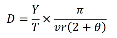
where 𝑌 is the number of detection events, 𝑇 is the total sampling time and 𝑣 is animal movement speed (or the distance travelled by an individual in a day); and 𝑟 and 𝜃, the mean radius and angle of the detection zone (i.e., the area within which animals are detected with certainty) are used to calculate the area of the detection zone (Nakashima et al., 2017; Pettigrew et al., 2021; Rowcliffe et al., 2008).
Independent estimates of 𝑣 can be sourced from telemetric studies, estimated from intensive observation or calculated using camera trap data (Nakashima et al., 2017, Rowcliffe et al., 2008, Rowcliffe et al., 2016). To calculate 𝑣 using camera traps: for each observation, practitioners should determine how long it took the animal to pass through the viewshed (i.e., time between first and last image in a sequence), then measure the distance the animal travelled by either a) retracing their path in the field using photos as a guide or b) estimating their movement image-to-image during photo processing using markers (Pfeffer et al., 2018, Rowcliffe et al., 2016).
𝑟 and 𝜃 can be measured in a few different ways. The first is by field trial: the detection zone is delineated by approaching the camera trap from different angles and at different speeds, recording where the sensor is triggered (Figure 7; Rowcliffe et al., 2008). The second is using a distance sampling method described in Rowcliffe et al. (2011). The third is by setting a focal area of standard size and shape (i.e., of known 𝑟 and 𝜃), within which detection is assumed to be perfect; only animals captured within the focal area are considered for analyses (Nakashima et al., 2017). 𝜃 may also be specified by the manufacturer (Pettigrew et al., 2021).
When the species of interest travels in packs or herds, density as calculated per the equation above represents group density (i.e., the number of groups per unit area; Rowcliffe et al., 2008). To convert group density to individual density, 𝐷 must be multiplied by an independent estimate of average group size (Rowcliffe et al., 2008).
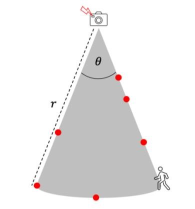
Clarke et al. (2023) - Fig. 7 Measuring 𝑟 and 𝜃 by field trial. The perimeter of the detection zone is determined by approaching the camera from different angles and at different speeds, and noting where the camera’s sensor (red flash) detects motion (red dots).
Simulations and Field Experiments (Clarke et al., 2023)
Of all the unmarked density models, the REM has undergone the most empirical testing (Palencia et al., 2021). Rowcliffe et al. (2008) piloted the model in an enclosed animal park housing populations of known sizes, and found that the REM produced accurate density estimates for three out of four target species (two cervids and a marsupial). The model underestimated the density of the fourth species (a large rodent) because cameras were deployed in habitats it did not frequent – a violation of assumption 3 (Rowcliffe et al., 2008).
The REM has proven robust in many study systems. Examples include:
Palencia et al. (2021) found that the REM yielded similar density estimates as two non-camera methods, line-transect sampling and drive counts, for red deer and wild boar, respectively. The researchers also compared the REM to two other camera methods (random encounter and staying time (REST) and distance sampling (DS) models) – of the three, the REM was the most consistent (Palencia et al., 2021). In this study, animal movement speed 𝑣 was determined using camera trap data.
REM-derived density estimates of a mountain ungulate were highly consistent with visual count survey results (Kavčić et al., 2021). Animal movement speed was measured using camera trap data (Kavčić et al., 2021).
A study on black bears in Québec found that the REM produced comparable results to DNA mark-recapture using hair samples, but that REM estimates were less precise (Pettigrew et al., 2021). The researchers estimated animal movement speed by averaging 19 years of telemetry data from four neighbouring black bear populations (Pettigrew et al., 2021).
In the boreal forest of Washington state, REM and live-trapping spatial capturerecapture (SCR) produced similar density estimates for snowshoe hare (Jensen et al., 2022). The REM and the REST performed identically in this system; both models outperformed the time-to-event (TTE) model (Jensen et al., 2022). Measures of animal movement speed 𝑣 were pulled from camera data and combined with telemetry data from a study in the Yukon.
The REM yielded similar density estimates as, and was more precise than, livetrapping SCR at almost 90% of sampling sites in a study of hedgehogs (Schaus et al., 2020). Moreover, the REM was powerful enough to detect a 25% population change in this system (Schaus et al., 2020). Animal movement speed was estimated from camera trap images.
The REM has also significantly over and underestimated the densities of natural populations. In Africa, for example, estimates of lioness density using the REM were significantly higher than from pride censuses (Cusack et al., 2015). REM-derived densities skewed high because cameras were placed under shady trees, which attracted lions in the daytime (a violation of assumption 3), inflating the number of detection events 𝑌 (Cusack et al., 2015). When only nighttime detections were considered, however, REM-derived densities did not differ significantly from censusderived densities (Cusack et al., 2015). 𝑣, animal movement speed, was determined via intensive observation. A study comparing the REM with fecal DNA mark-recapture found that the REM underestimated marten density by 60% or more (Balestrieri et al., 2016). Animal movement speed 𝑣 may have biased density low; the researchers estimated 𝑣 from studies of pine marten occupying a different kind of habitat, where individuals may have moved more (Balestrieri et al., 2016).
Simulations suggest that, to achieve adequate precision using the REM, a minimum of 20 to 40 camera stations should be deployed for as long as needed to collect at least 10 to 20 image sets (Rowcliffe et al., 2008). For populations with variable detection: about 100 cameras are needed to obtain a level of precision appropriate for wildlife management (coefficient of variation (CV) of 0.20 or less; Palencia et al., 2021, Williams et al., 2002). To collect 10 to 20 image sets takes approximately 100 to 1,000 camera trap days for most mammal species; for rare species, cameras may need to be deployed for 1,000 camera trap days or more (Rowcliffe et al., 2008).
Visual resources
Clarke et al. (2023) - Fig. 7 Measuring 𝑟 and 𝜃 by field trial. The perimeter of the detection zone is determined by approaching the camera from different angles and at different speeds, and noting where the camera’s sensor (red flash) detects motion (red dots).
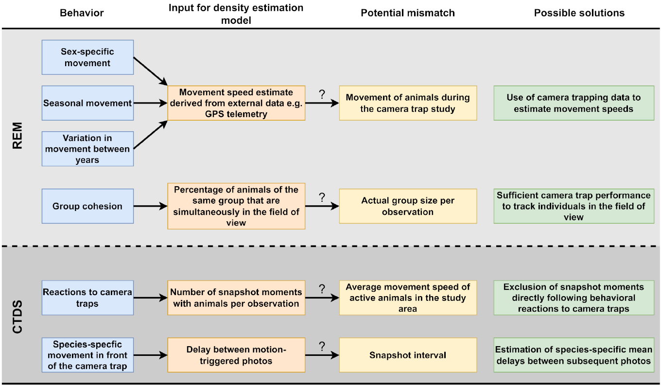
Henrich et al. (2022) - Fig. 1 Potential problems caused by animal behavior in the estimation of population densities of unmarked animal species using camera traps and our proposed solutions.
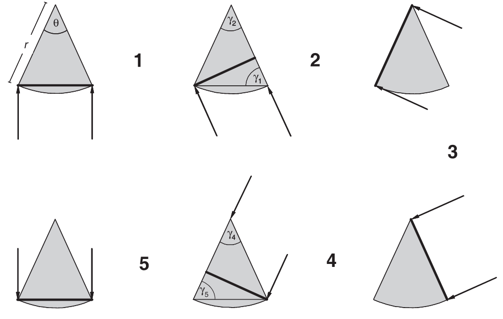
Rowcliffe et al. (2008) - Fig. 1 Diagram illustrating the variation in profile presented to animals approaching from different angles by a segment-shaped camera trap detection zone.
Approach directions are indicated by arrows, the detection zone is the shaded segment, defined by radial distance r and angle θ, and the profiles presented are indicated by heavy lines. Six limiting cases are shown for π approach angles, with five resulting transitions. The angles opposite the profiles, γ, are indicated for transitions 1, 2, 4 and 5 (the profile for transition 3 is constant so no such angle is required). The widths of profiles and ranges of γ for each transition are given by: transitions 1 and 5, 2r sin(θ/2) sin(γ), (π – θ)/ 2 ≤ γ ≤ π/2; transitions 2 and 4, r sin(γ), θ ≤ γ ≤ π/2; transition 3, r for θ approach angles.
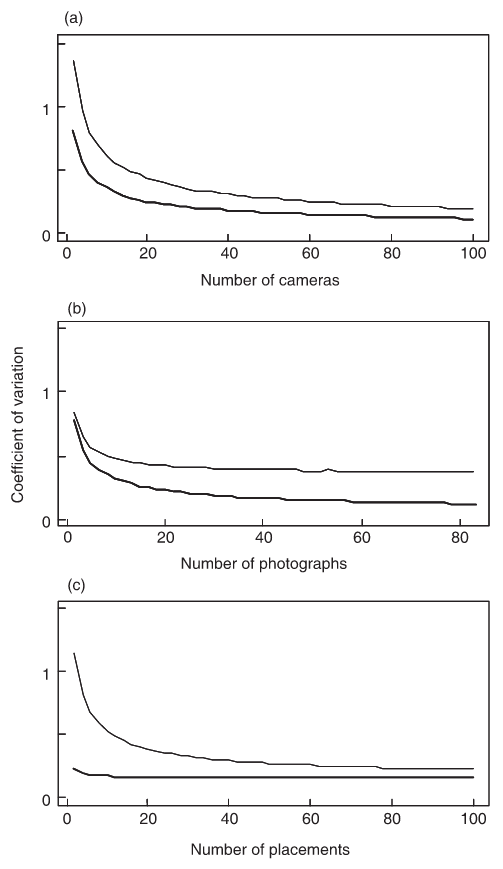
Rowcliffe et al. (2008) - Fig. 4 The precision of estimated density from simulated data in relation to variation in sampling effort, assuming high or low variance in camera trapping rate (upper and lower curves, respectively, in each graph).
Effort is varied as either (a) the number of cameras while holding time per camera constant; (b) the time per camera (indexed by the total number of photographs taken) while holding the number of cameras constant; and (c) the number of camera placements while holding the total amount of camera time constant.
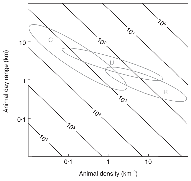
Rowcliffe et al. (2008) - Fig. 5 Expected trapping effort (camera days, indicated by contours) required to achieve 10 photographs given varying density and day range, assuming a group size of 1.
Typical combinations of day range and density are indicated for carnivores (C), ungulates (U) and rodents (R), calculated using allometric equations for day range and density at carrying capacity (see text) and illustrating densities between 10% and 100% of carrying capacity.
Camera Trap Methods for Density Estimation
Shiny apps/Widgets
Check back in the future!
Analytical tools & Resources
Type |
Name |
Note |
URL |
Reference |
|---|---|---|---|---|
References