Space-to-event (STE)#
Assumptions, Pros, Cons
Demographic closure (i.e., no births or deaths) (Moeller et al., 2018)
Geographic closure (i.e., no immigration or emigration) (Moeller et al., 2018)
Spatial counts of animals in a small area (or counts in equal subsets of the landscape) are Poisson-distributed (Loonam et al., 2021b)
Detection is perfect (detection probability ‘p’ = 1) (Moeller et al., 2018)
Can be efficient for estimating abundance of common species (with a lot of images) (Moeller et al., 2018)
Does not require estimate of movement rate (Moeller et al., 2018)
Detection is perfect (detection probability ‘p’ = 1) (Moeller et al., 2018)
This section will be available soon! In the meantime, check out the information in the other tabs!
Note
This content was adapted from: The Density Handbook, “Using Camera Traps to Estimate Medium and Large Mammal Density: Comparison of Methods and Recommendations for Wildlife Managers” (Clarke et al., 2023)
The space-to-event model (STE) is an extension of the time-to-event model (TTE; see Time-to-event) that measures the area, instead of the time, sampled before an image of an animal is observed (Moeller et al., 2018). The conceptual underpinnings of the STE are the same as those of the TTE, with the exception that sampling occasions are collapsed into instantaneous samples using time-lapse images – photographs taken at predetermined periods of the day or night (e.g., every hour, every day at noon), regardless of whether animals are within frame (Figure 12; Granados, 2021; Moeller et al., 2018). Because they are collapsed into instants in time, there is no need to break sampling occasions down into sampling periods – and no need for measures of animal movement speed.
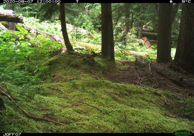
Clarke et al. (2023) - Fig. 12 One of many time-lapse images taken at a camera station at noon. Notice, the camera trap captures an image at a predetermined time (12:00), regardless of whether an animal is within frame.
The STE model is based on the simple logic that, as population density increases, the number of animal images captured by the cameras in a network increases, and thus the number of cameras that capture images increases – so, at a moment in time, the number of cameras from which images need to be “drawn” until an image of an animal is picked decreases (Lukacs, 2021). To visualize how to model works: say an array of camera traps is deployed randomly across a study landscape, and set to take images every hour, on the hour (i.e., hourly sampling occasion). After image collection, for each occasion, images are “drawn” from cameras in random order, until an image of an animal is picked (Moeller et al., 2018). An example encounter history after 7 sampling occasions (e.g., 7 hours), for which the average viewshed area 𝑎 is 20 m2, might look like: {NA, 40 m2, NA, NA, 1180 m2, NA, 800 m2}, where 40 m2 indicates that images from 2 cameras had to be drawn before observing an animal, 1180 m2 indicates images from 59 cameras had to be drawn, and so on; and NA indicates no animal detections for that occasion. This encounter history – which summarizes the space until detections – can then be plugged into a modified TTE equation to produce a density estimate (Moeller et al., 2018).
As with the TTE, the average area of a camera viewshed is calculated using the equation:
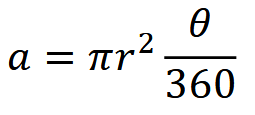
where 𝑟 is detection distance and 𝜃 is the angle of the camera lens in degrees (Moeller et al., 2018). 𝑟 – instead of being the maximum distance at which an animal can trigger a camera’s motion sensor, however, as it is for the TTE – is simply the maximum distance at which an animal is identifiable, and is measured using landmarks as references (Gilbert et al., 2020; Moeller et al., 2018).
Simulations and Field Experiments
Random walk simulations show that the STE – unlike the TTE – is insensitive to movement speed (Moeller et al., 2018). This means that the model produces unbiased estimates of density, whether animals move slowly or quickly. The STE has been field-tested on high-density ungulates and low-density carnivores in Idaho:
In Idaho, the STE produced an estimate of elk density comparable to an aerial survey and the TTE (Moeller et al., 2018). The precision of STE and TTE estimates was similar in this system.
For wolves – a low-density, social species – the STE yielded densities close to those from a parallel DNA mark-recapture study (Ausband et al., 2022). STEderived results were less precise, however. Density was also significantly overestimated during one survey period (before data transformation) because of high detection rates at a single camera (Ausband et al., 2022). The researchers recommended bootstrapping (i.e., resampling a data set with replacement) to correct estimates when a camera collects too few or too many images.
The model performed comparatively poorly for low-density, solitary cougars; STE estimates were less precise and more variable than those from genetic markrecapture and the random encounter model (REM; see Random encounter model; Loonam et al., 2021a). Small sample sizes (i.e., few occasions with images of cougars) contributed to the STE’s inconsistency (Loonam et al., 2021a). It is worth noting, however, that genetic mark-recapture-based estimates were also fairly inconsistent, and density was not calculable during some surveys due to a lack of recaptures, despite considerable field effort (Loonam et al., 2021a). The STE may therefore still be an efficient alternative to DNA markrecapture.
Moeller & Lukacs (2021) The spaceNtime workflow for count data. The user will go through five major steps for STE, TTE, and IS analyses. If the user has presence/absence (0 and 1) data instead of count data, the IS analysis is not appropriate, and the IS pathway should be removed from the flowchart
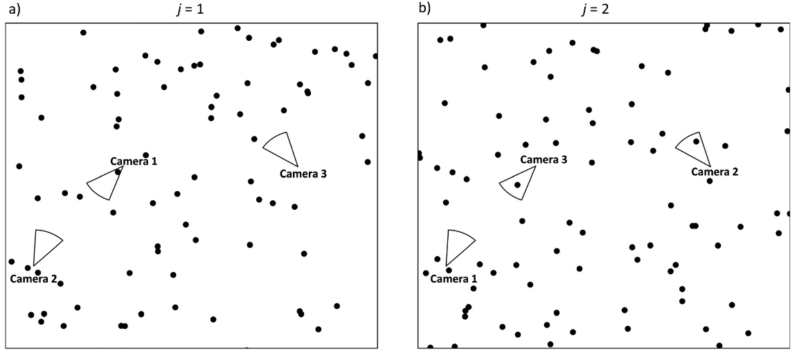
Moeller et al. (2018) - Fig. 3 Conceptual diagram of the space to event (STE) model.
The circular sectors represent three different cameras on two different occasions (a-b). On each occasion j = 1, 2,…, J, we randomly order the cameras i = 1, 2,…, M. If the first animal detection is in the nth camera, the observed STE Sj is the sum of the areas of cameras 1, 2,. .. n. (a) On occasion j = 1, camera 1 contains at least one animal, so we record the space to first event S*j*=1 = a1. (b) On occasion j = 2, cameras 2 and 3 both contain animals, but we use the first camera in the series. Therefore, we record the space to first event Sj=1 = a1 + a2.
Clarke et al. (2023) - Fig. 12 One of many time-lapse images taken at a camera station at noon. Notice, the camera trap captures an image at a predetermined time (12:00), regardless of whether an animal is within frame.
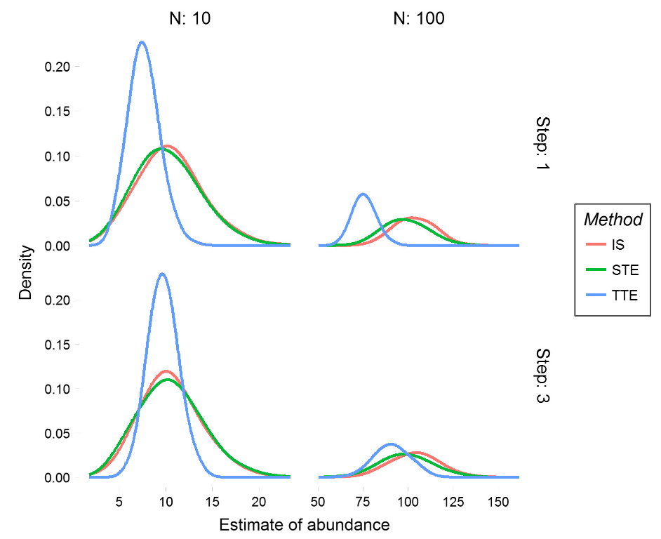
Moeller et al. (2018) - Fig. 4 Abundance estimates from simulated populations.
We performed 1000 simulations for each of the three models at two step lengths for populations of size 10 (left column) and 100 (right column). Simulated animals took an uncorrelated random walk with step length 1 for the slow populations (top row) and step length 3 for the fast populations (bottom row).
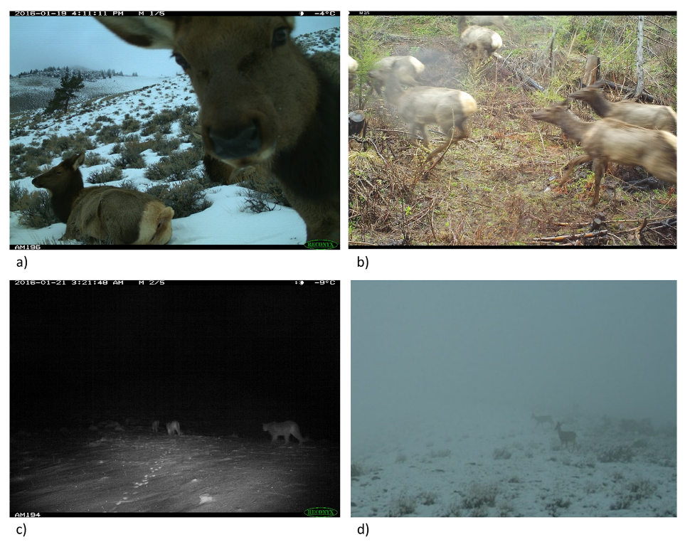
Moeller et al. (2018) - Fig. 7 Factors that influence accurate group counts.
Various factors can influence accurate counts of group size, including animal behavior (a, b), photograph quality (c), and weather (d). Although it may be difficult to accurately count group size in these four photographs, the species is still identifiable. In studies where group counts are consistently difficult but species identification is possible, the space to event model is a useful tool to estimate abundance.


Check back in the future!
Type |
Name |
Note |
URL |
Reference |
|---|---|---|---|---|
R package |
spaceNtime: an R package for estimating abundance of unmarked animals using camera-trap photographs |
free and open-source R package designed to assist in the implementation of the STE and TTE models, along with the IS estimator |
<annam21/spaceNtime |
Ausband, D. E., Lukacs, P. M., Hurley, M., Roberts, S., Strickfaden, K., & Moeller, A. K. (2022). Estimating Wolf Abundance from Cameras. Ecosphere, 13(2), e3933. https://doi.org/10.1002/ecs2.3933
Clarke, J., Bohm, H., Burton, C., Constantinou, A. (2023). Using Camera Traps to Estimate Medium and Large Mammal Density: Comparison of Methods and Recommendations for Wildlife Managers. https://doi.org/10.13140/RG.2.2.18364.72320
Gilbert, N. A., Clare, J. D. J., Stenglein, J. L., & Zuckerberg, B. (2020). Abundance Estimation of Unmarked Animals based on Camera-Trap Data. Conservation Biology, 35(1), 88-100. https://doi.org/10.1111/cobi.13517
Granados, A. (2021). “WildCAM Guide to Camera Trap Set Up.” WildCAM. https://wildcams.ca/site/assets/files/1148/wildcam_guide_to_camera_trap_set_up_feb2021.pdf
Loonam, K. E., Ausband, D. E., Lukacs, P. M., Mitchell, M. S., & Robinson, H. S. (2021a). Estimating Abundance of an Unmarked, Low‐Density Species using Cameras. The Journal of Wildlife Management, 85(1), 87-96. https://doi.org/10.1002/jwmg.21950
Loonam, K. E., Lukacs, P. M., Ausband, D. E., Mitchell, M. S., & Robinson, H. S. (2021b). Assessing the robustness of time-to-event models for estimating unmarked wildlife abundance using remote cameras. Ecological Applications, 31(6), Article e02388. https://doi.org/10.1002/eap.2388
Lukacs, P. M. (2021, Oct 26).Animal Abundance from Camera Data:Pipe Dream to Main Stream. Presented at the FCFC Seminar. https://umontana.zoom.us/rec/play/eY6_CAjDNUjCAfFrmRvJH8NtrL4J38I46T5idY4gO3i1YHqxBnDUrDeufvgAps-D-aFJFJ_F9AMuE6k.VjerQ5kRpa5HsybV
McMurry, S., Moeller, A. K., Goerz, J., & Robinson, H. S. (2023). Using space to event modeling to estimate density of multiple species in northeastern Washington. Wildlife Society Bulletin, 47(1). https://doi.org/10.1002/wsb.1390
Moeller, A. K.,& Lukacs, P. M. (2021) spaceNtime: an R package for estimating abundance of unmarked animals using camera-trap photographs. Mammalian Biology, 102, 581-590. https://doi.org/10.1007/s42991-021-00181-8
Moeller, A. K., Lukacs, P. M., & Horne, J. S. (2018). Three Novel Methods to Estimate Abundance of Unmarked Animals using Remote Cameras. Ecosphere, 9(8), Article e02331. https://doi.org/10.1002/ecs2.2331