Time-to-event (TTE)#
Assumptions, Pros, Cons
Demographic closure (i.e., no births or deaths) (Moeller et al., 2018; Loonam et al., 2021b)
Geographic closure (i.e., no immigration or emigration) at the level of the sampling frame (area of interest); this assumption does not apply at the plot-level (area sampled by the camera) (Moeller et al., 2018; Loonam et al., 2021b)
Animal movement and behaviour are unaffected by the cameras (Palencia et al., 2021)
Camera locations placement is random, systematic, or systematic random (Moeller et al., 2018)
Spatial counts of animals (or counts in equal subsets of the landscape) are Poisson-distributed (Loonam et al., 2021b)
Inaccurate estimate of movement speed (Loonam et al., 2021b)
Detection is perfect (detection probability ‘p’ = 1) (Moeller et al., 2018)
Can be efficient for estimating abundance of common species (with a lot of images) (Moeller et al., 2018)
Requires independent estimates of movement rate (difficult to obtain without telemetry data) (Moeller et al., 2018)
This section will be available soon! In the meantime, check out the information in the other tabs!
Note
This content was adapted from: The Density Handbook, “Using Camera Traps to Estimate Medium and Large Mammal Density: Comparison of Methods and Recommendations for Wildlife Managers” (Clarke et al., 2023)
Time-to-event (TTE) analysis is used in many disciplines to estimate the rate at which an event occurs, by repeatedly measuring the time that elapses before said event takes place (Loonam et al., 2021b). A TTE model might be used in medicine, for example, to approximate time from diagnosis until remission or death (Clark et al., 2003). Moeller et al. (2018) developed an extension of the TTE framework to estimate animal density using camera trap data, where the “event” of interest is an animal detection, and the rate of interest is animals per viewshed area – density (Loonam et al., 2021b). Their version capitalizes on the fact that, at a randomly deployed motion-triggered camera, the time it takes to capture an image of an animal is a function of animal movement speed, detection probability and population size (Jennelle et al., 2002; Moeller et al., 2018; Parsons et al., 2017). When movement speed is known and detection probability is perfect, population size can be estimated by measuring the time from an arbitrary starting point until an image of an animal is captured (Lukacs, 2021; Moeller et al., 2018).
The equation for camera data-based density estimation using TTE is:
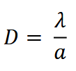
where 𝜆 is the average number of animals in the viewshed, given the time until an animal is detected, and 𝑎 is the average viewshed area. 𝑎 is calculated using the equation:
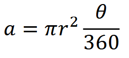
where 𝑟 is the trigger distance (i.e., the maximum distance from which an animal can reliably trigger a camera’s motion sensor), and 𝜃 is the angle of the camera lens in degrees (Moeller et al., 2018).
To illustrate how 𝜆 is calculated, let’s take a simple example. We begin by dividing the total time cameras are active into sampling occasions, then sampling periods (Figure 10; Moeller et al., 2018). We might choose to define a sampling occasion as a day, and a sampling period as one of 24 one-hour intervals in a day (Moeller et al., 2018). The images collected at a camera station can now be grouped by occasion and period to generate a detection history, and the number of sampling periods (i.e., 𝑘 out of 24) until an image of an animal is encountered can be determined for each sampling occasion (Moeller et al., 2018). The detection history at a given camera after 7 days might look something like {NA, NA, 7, NA, 22, 1, NA}, where NA indicates no animal detections for that day. Inputting this information into a likelihood equation generates the average number of animals in the viewshed, 𝜆 (Moeller et al., 2018).
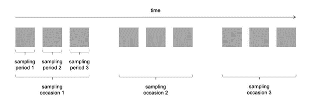
Clarke et al. (2023) - Fig. 10 Adapted from Moeller et al. (2018). Visualization of how total sampling time at a camera station is broken down into sampling occasions and then sampling periods.
To account for movement, the sampling period is set as the average time animals take to pass through the camera viewshed (Moeller et al., 2018). Thus, practitioners need measures of animal movement speed.
Simulations and Field Experiments
Simulations show that
The TTE model tends to underestimate population density. In both walk (Loonam, 2019) and random walk simulations (Moeller et al., 2018), the TTE yielded density estimates below the true value, whether populations were large or small, or animals moved quickly or slowly. Estimates were, however, particularly low for slow-moving species.
The TTE is sensitive to movement speed. Indeed, Loonam et al.’s (2021b) simulations showed that over- or underestimating movement rate biases density estimates. For example: a 50% underestimation of movement speed resulted in a density estimate 40% lower than the true density; overestimating movement speed by 200% resulted in density estimates that were over 85% higher than actual (Loonam et al., 2021b). Taken together, these results suggest that the integrity of TTE estimates depends on the movement behaviour of the focal species, and obtaining accurate measures of animal movement speed.
The TTE model performs best when cameras are deployed randomly on the landscape. Setting cameras to maximize detections (i.e., targeted deployment) resulted in considerable over- or underestimates of density in walk simulations (Loonam et al., 2021b). Of the sampling designs tested in Grosklos’ (in preparation) simulations, random camera placement produced the best results. Thus, practitioners using the TTE model are advised to deploy their camera networks randomly to minimize model bias.
The TTE is robust to population openness and territoriality. Population openness is a violation of assumption 1 (population closure); territoriality is a violation of assumption 5 (animals are Poisson distributed across the landscape; Moeller et al., 2018). Neither appeared to impact TTE estimates – indicating that the model applies well to actual populations, which often violate these assumptions (Loonam et al., 2021b).
It is worth noting that in all of Loonam et al.’s (2021b) simulations, the precision of TTE estimates was inflated – that is, estimates were calculated to be more precise than they actually were. Practitioners should keep this in mind when evaluating reported values of precision, as they may be artificially high.
In the field
the TTE has produced density estimates similar to established censusing techniques. Moeller et al., (2018) piloted the TTE on a population of elk in Idaho, and found that the model produced a density estimate comparable to an aerial survey of the same area – even though cameras were not deployed randomly. In this system, the TTE produced higher estimates of population density than either of its sister models (space-to-event (STE) and instantaneous sampling (IS); see below). For cougars – a low-density species – TTE-based estimates were actually more precise than both genetic mark-recapture and random encounter model (REM; see Random encounter model [REM]) estimates, and similarly or more consistent across years, respectively (Loonam et al., 2021a). Density estimates could have been biased and misleadingly precise, however, because of non-random camera placement (Loonam et al., 2021a, Morin et al., 2022).
The TTE has also performed poorly in natural populations. A study on snowshoe hare found that the TTE tended to overestimate density compared with the REM and the random encounter and staying time model (REST; see Random encounter and staying time [REST]; Jensen et al., 2022). Out of the three camera-based models, the TTE was also the least consistent with live-trapping spatial capture-recapture (SCR; see Spatial capture-recapture (SCR) / Spatially explicit capture recapture (SECR); Jensen et al., 2022)
Clarke et al. (2023) - Eqn TTE:
The equation for camera data-based density estimation using TTE, where 𝜆 is the average number of animals in the viewshed, given the time until an animal is detected, and 𝑎 is the average viewshed area.
Clarke et al. (2023) - Eqn TTE 𝑎:The equation for 𝑎 in camera data-based density estimation using TTE (refer to “Clarke et al. (2023) - Eqn TTE”).
Clarke et al. (2023) - Fig. 10 Adapted from Moeller et al. (2018). Visualization of how total sampling time at a camera station is broken down into sampling occasions and then sampling periods.
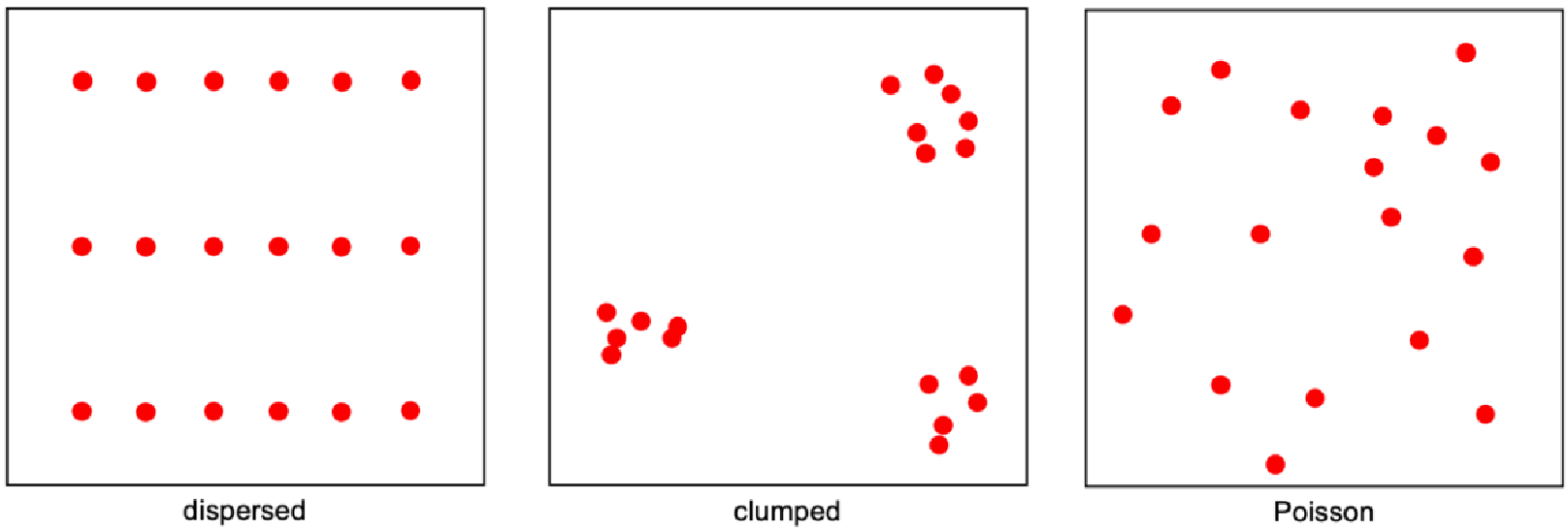
Clarke et al. (2023) - Fig. 11 Simple diagrams showing dispersed, clumped and Poisson-distributed animals (red dots) in space.
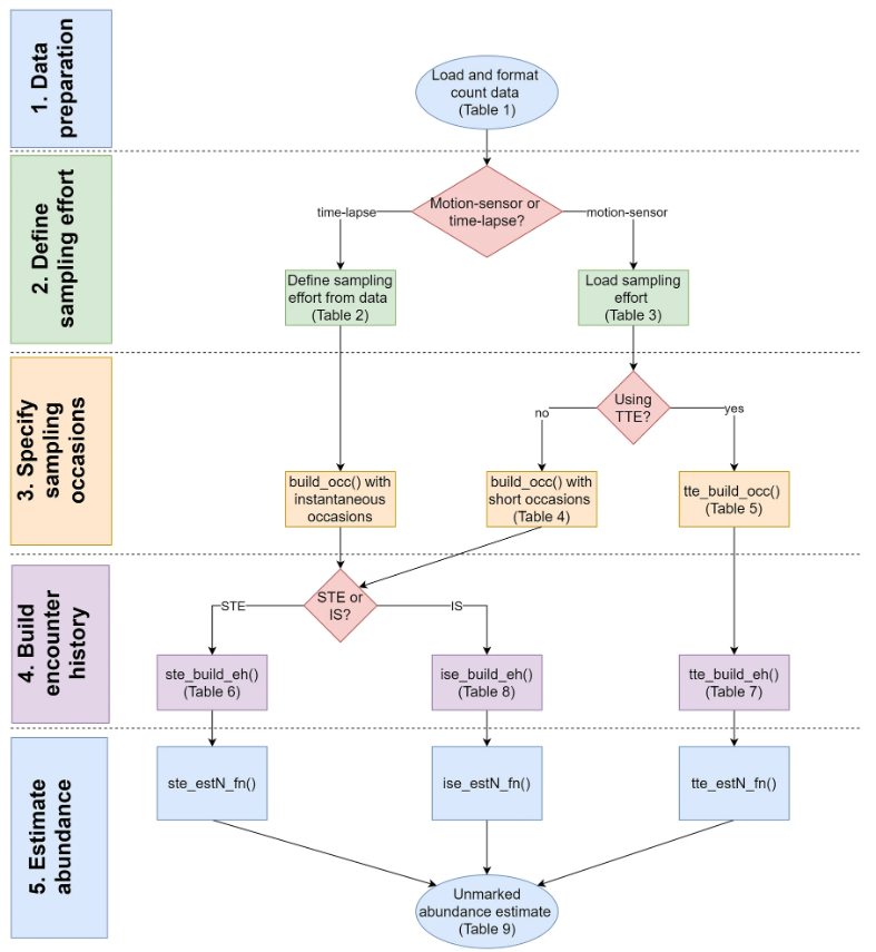
Moeller & Lukacs (2021) The spaceNtime workflow for count data. The user will go through five major steps for STE, TTE, and IS analyses. If the user has presence/absence (0 and 1) data instead of count data, the IS analysis is not appropriate, and the IS pathway should be removed from the flowchart.
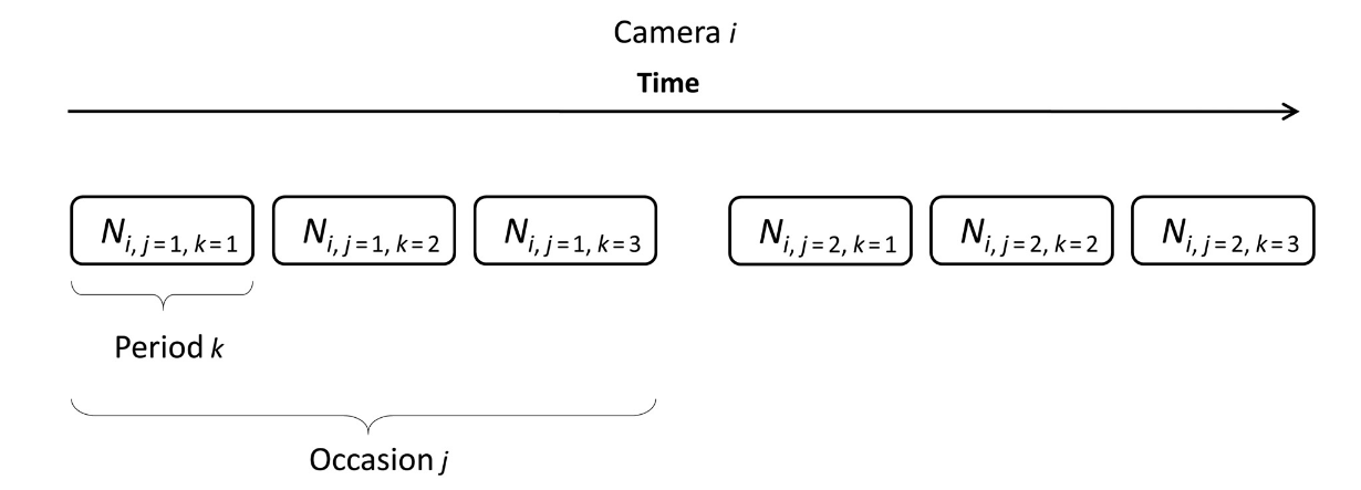
Moeller et al. (2018) - Fig. 1 Schematic of sampling periods and occasions for the time to event model. At camera i = 1, 2, …, M, sampling occasion j = 1, 2, …, J is broken into several sampling periods k = 1, 2, …, K. Here, J = 2 and K = 3.
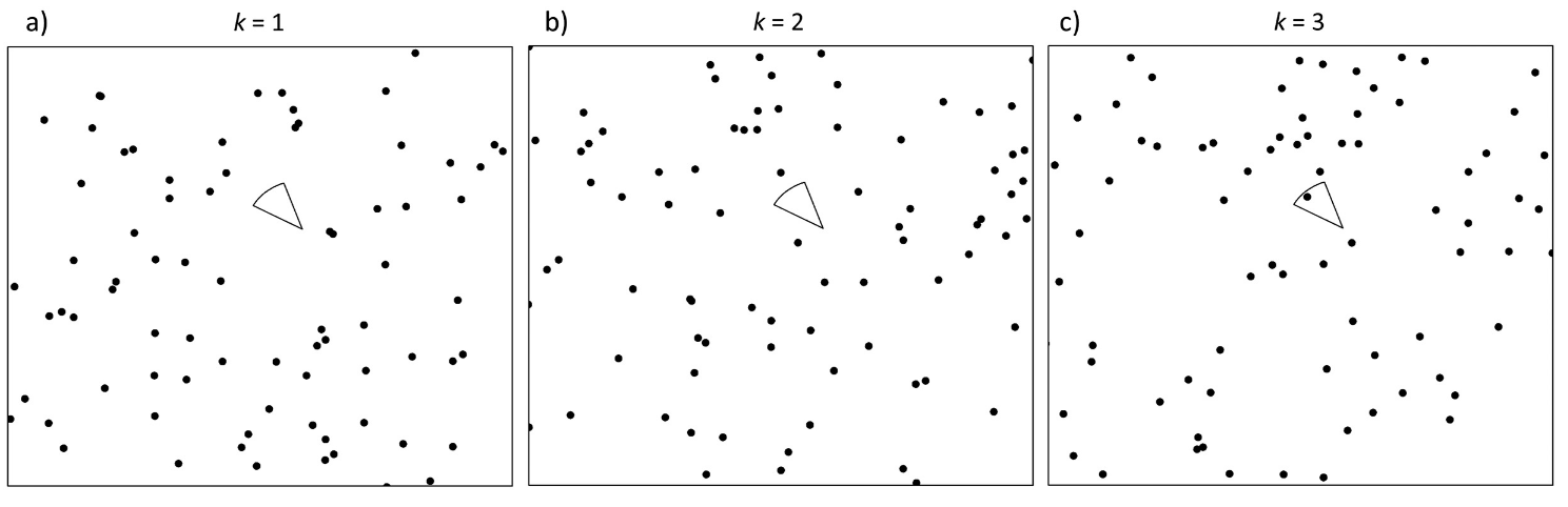
Moeller et al. (2018) - Fig. 2 Conceptual diagram of the time to event (TTE) model.
The circular sector is the viewshed of a single camera i on a single occasion j divided into three successive sampling periods (a–c). The black dots represent randomly placed animals. The observed TTE Tij is equal to the period k in which the camera first contains an animal. There are no animals in the camera in (a) k = 1 or (b) k = 2, but there is an animal in the camera in (c) k = 3, so for this camera and sampling occasion, T*ij* = 3.

Check back in the future!
Type |
Name |
Note |
URL |
Reference |
|---|---|---|---|---|
R package |
spaceNtime: an R package for estimating abundance of unmarked animals using camera-trap photographs |
A free and open-source R package designed to assist in the implementation of the STE and TTE models, along with the IS estimator. |
annam21/spaceNtime; |
Moeller, A. K.,& Lukacs, P. M. (2021) spaceNtime: an R package for estimating abundance of unmarked animals using camera-trap photographs. Mammalian Biology, 102, 581-590. https://doi.org/10.1007/s42991-021-00181-8 |
(