6.0 Study design

6.0 Study design#

Project or survey-level aspects of design that camera users should consider (at a minimum) are:

Study area extent and method of delineation (e.g., watershed or minimum convex polygon)
Criteria for site selection (e.g., random, systematic, or targeted habitat types or features)
Camera arrangement (e.g., random vs. cameras ‘clustered’ into hierarchical groups with common characteristics)’ into hierarchical groups with common characteristics)
Camera spacing (e.g., 1 km spacing between cameras) km spacing between cameras)
Number (or density) of cameras
Survey effort and timing (i.e., the number of days the camera was active and functioning during the survey period; the “camera days per camera location,“ the total number of camera days, time of year, and survey duration)

These decisions will depend on the study objectives as well as the resources available.

Decisions concerning study design are a critical component of any wildlife project. These decisions can be complex, and in these cases, it is highly advisable to consult an expert for direction.

6.1 Study area#

A study area is a unique area(s) within a project. There may be multiple study areas within a larger study area. Aspects to consider when identifying the study area include the spatial extent (and method of delineation), shape (Foster & Harmsen, 2012), and composition and configuration of features within it (including habitat types, land uses and disturbances).

Several factors influence the size (spatial extent) of the study area, including the objectives, ecosystem, the biology of the Target Species (e.g., dispersal ability, habitat preferences, etc.) and/or modelling approach.

For example, density models using the capture-recapture (CR) modelling approach requires that the study area encompasses the entire area in which individuals can move during the survey and that each individual can be detected by a camera (Karanth & Nichols, 1998). In this case, the animal’s home range size could be used (e.g., four times the home range size [Maffei & Noss, 2008]) (Wearn & Glover-Kapfer, 2017) in combination with a finite number of cameras available (e.g., 20 cameras are available; ideally, they should be paired and there should be > 4 cameras in each home range [Wearn & Glover-Kapfer, 2017]) to define the project’s spatial extent.

Methods to delineate the appropriate spatial extent include, for example, minimum convex polygons (i.e., a polygon surrounding the locations of previous detections) or kernel density estimators (e.g., via the probability of “utilization” [Jennrich & Turner, 1969]). Geographic Information Systems (GIS, e.g., ESRI software) or programming languages (e.g., R) contain useful tools for these delineation methods.

6.2 Site selection and camera arrangement#

Remote camera locations (or sample stations) and their spatial arrangement are integral components of any study design; these choices will affect the user’s ability to draw inference(s) about the species or question of interest. There are many species-specific characteristics (e.g., body size, behaviour, rarity, etc.) and environmental factors (e.g., vegetation cover, snow depth) that influence the detection probability and probability of occurrence of a species, as well as the size of the area that should be surveyed (e.g., Becker et al., 2022; Hofmeester et al., 2019; Iknayan et al., 2014; Steenweg et al., 2019). When there are multiple Target Species, a mix of study designs may be valuable (Iannarilli et al., 2021; van Wilgenburg et al., 2020).

The objectives of the survey will determine the most appropriate study design (Appendix A - Table A2). There are five commonly used study designs in camera studies: simple random, systematic random (grid), stratified random, clustered (including paired design) and targeted (or opportunistic) (Wearn & Glover-Kapfer 2017). A convenience sampling study design is also used when it is impractical to use another design. Sampling design can occur hierarchically, where one approach is used at a larger scale (i.e., to select grids to place cameras within), and another approach is used at a smaller scale (i.e., to select the location within each grid to place the camera). Refer to the following literature for additional recommendations on study design: Burton et al., 2015; Cusack et al., 2015; Fisher & Burton, 2012; Kolowski and Forrester, 2017; Meek et al., 2014b; O’Connell et al., 2011b; Rovero et al., 2013; Steenweg et al., 2015; Wearn & Glover-Kapfer, 2017 and WildCAM’s “sampling design & effort section section” of their resource library (https://wildcams.ca/library/camera-trapping-papers-directory/).

Note that we refer to different configurations of cameras more generally as study design and sampling design; however, the term “Survey Design“ is how the study design is referred to when it applies to an individual survey. There may be multiple Survey Designs for surveys within a project; the Survey Design should be reported separately for each survey within a project. When the Survey Design is hierarchical, “Hierarchical (multiple)*” should be reported and additional details should be included in the Survey Design Description. Refer to the AB Metadata Standards (RCSC, 2024) for more information.

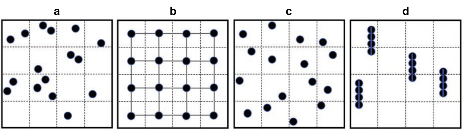
../_images/Survey-guidelines_CamConfig.png

Figure 3. Examples of sampling designs: (a) simple random, (b) systematic, (c) stratified (each grid cell is a stratum), and (d) clustered (adapted from Schweiger, 2020).

6.2.1 Random (or “simple random”) design#

Random (or “simple random”) design (Figure 3a) – cameras occur at randomized locations (or sample stations) across the study area, sometimes with a predetermined minimum distance between camera locations (or sample stations). A random design may help reduce biases that arise from selecting camera locations deliberately. It may also allow the user to make inferences about areas that were not surveyed when employing use-based approaches (e.g. occupancy models [MacKenzie et al., 2002]; intensity of use methods [Keim et al., 2019]). Some modelling approaches (e.g., random encounter and staying time [REST]; Nakashima et al., 2018) and [random encounter models REM; Rowcliffe et al., 2008, 2013]) require a simple random design ([Appendix A - Table A2](/1_survey-guidelines/1_10.1_AppendixA-Tables.md#TOC_surv_guidelines_table_aurv_guidelines_table_advantage of using a simple random design is the tendency to see fewer animals (i.e., is less efficient) when animals are clustered or exhibit habitat preferences, and the possibility of missing rare habitat types. The proportion of different strata (e.g., habitat types) sampled should be the same as (or close to) the true proportion in the study area. For example, if the study area consists of 25% young deciduous forest, then 25% of randomly selected sites should be within young deciduous forest, on average.

6.2.2 Systematic design#

Systematic design (Figure 3b) – camera locations occur within a regular pattern (e.g., a grid pattern) across the study area.

Systematic random – camera locations are selected using a two-stage approach. Firstly, grids are selected systematically (to occur within a regular pattern) across the study area. The location of the camera within each grid is then selected randomly. This method is similar to the simple random design. The same advantages apply in terms of unbiased landscape representation, and the same modelling approaches can be used. The disadvantage of using a systematic random (or simple random design) is that rare habitat types may be missed.

Systematic non-random design – sets of clustered cameras can be deployed within a systematic non-random approach (i.e., “systematic clustered” or “systematic paired”) to assess the effects of disturbance along a gradient, over time, at multiple scales and/or with control (i.e., reference) sample stations. Hierarchical Before-After Dose-Response (BADR) is one such method that requires cameras to be placed within a systematic non-random approach, where camera locations occur along transects or in clustered arrays (sample stations), selected using a nested spatial hierarchy of sampling to control for variability in land-use type and large-scale patterns (Bayne et al., 2022). The study area is divided into land-use regions based on land-use type, then into landscape units, which are assessed for environmental variability to determine where sample stations should be placed (Bayne et al., 2022). The “Before-After” component of BADR incorporates the phase of stressors (i.e., proposed or current development) (Bayne et al., 2022). The “Dose-Response” component of BADR controls for the variable distribution of activity (and the potential impacts) by incorporating control (or reference) sample stations and/or by placing cameras in sample stations along a gradient of disturbance (Bayne et al., 2022).

6.2.3 Stratified design#

Stratified random design (Figure 3c) – the area of interest is divided into smaller strata (e.g., habitat type, disturbance levels), and then a proportional random sample of sites is selected within each stratum (e.g., 15%, 35% and 50% of sites within high, medium and low disturbance strata). This design can help ensure that the sample adequately reflects the major or uncommon strata of interest and may be an efficient approach when users are limited by accessibility constraints (Wearn & Glover-Kapfer, 2017). This design can also be used to increase precision if animal densities are known to be highly variable (Junker et al., 2021) or when a species is expected to occur in certain habitat types more often (Gillespie et al., 2015). For example, studies that wish to assess species richness, or occupancy rates for a particular species, amongst strata would use a stratified random design.

6.2.4 Clustered / Paired designs#

Clustered design (Figure 3d) – multiple cameras are deployed at a sample station. The distance between cameras (camera spacing) will be influenced by the chosen sampling design, the Survey Objectives, the Target Species and data analysis. A clustered design can be used within a systematic or stratified approach (i.e., systematic clustered design or as a clustered random design) (Wearn & Glover-Kapfer, 2017). A clustered design is common when users are interested in individual identification, such as density estimation from marked or partially marked populations (e.g., [spatially explicit capture-recapture SECR; Borchers & Efford, 2008; Efford, 2004; Royle & Young, 2008] or [spatial mark-resight SMR; Doran-Myers, 2018]). A clustered design can also be used in an occupancy framework (O’Connell & Bailey, 2011; Pacifici, 2015) when interested in measures of species richness (O’Brien et al., 2011).

A clustered design can be a cost-efficient approach to increase the number of replicates at each site (especially when accessibility is limiting; Gálvez et al., 2016) and to reduce measurement error and improve precision (Clarke et al., 2019). However, spatial autocorrelation may occur with this design (Moqanaki et al., 2021), depending on the camera spacing (see section 6.2.7).

Paired design – a form of “clustered design“ where two cameras that are placed closely together to increase detection probability (“paired cameras”), to evaluate certain conditions (“paired sites,” e.g., on- or off trails), etc. Paired placements can help to account for other variability that might occur (i.e., variation in habitat quality). For some objectives, pairs of cameras might be considered subsamples within another sampling design (e.g., simple random, stratified random, systematic).

6.2.5 Targeted design#

Targeted design – cameras are placed in areas that are known or suspected to have higher activity levels (e.g., game trails, mineral licks, etc.). This design is useful when monitoring rare or cryptic species that are unlikely to be detected with other designs. This design is commonly used when estimating densities of marked populations (e.g., [spatially explicit capture-recapture SECR; Borchers & Efford, 2008; Efford, 2004; Royle & Young, 2008]) or behaviour studies. It is, however, important to understand that targeted sampling may impede one’s ability to make inferences beyond the survey area. For some objectives, targeted sampling may be used within another sampling design (e.g., a stratified random sample of game trails and seismic lines; Keim et al. 2021).

6.2.6 Convenience design#

Convenience design – camera locations or sample stations are chosen based on logistic considerations (e.g., remoteness, access constraints, costs). When cost is a key consideration, other more rigorous sampling designs (e.g., stratified; van Wilgenburg et al., 2020) that can incorporate cost should be considered first. One should be cautious when generalizing or drawing conclusions from data collected using convenience sampling, given that estimates can be biased if the sample poorly represents the population of interest. The convenience sampling design can be used where the goal is to survey a specific location(s) without the intent to generalize to un-surveyed areas (Gillespie et al., 2015; e.g., Kusi et al., 2020) or to survey an area following a report of the occurrence of a rare species. Both randomized (e.g., Found & Patterson, 2020) or targeted approaches can be used within a convenience sampling approach, although the user should still be cautious about extrapolating inferences to areas (or habitat types in an occupancy framework [MacKenzie et al., 2002]) that were not sampled and, therefore, not represented in the data (Gillespie et al., 2015).

6.2.7 Pseudoreplication#

Spatial autocorrelation (i.e., the tendency for sites that are close together to be more similar) may occur when multiple cameras are placed nearby (such as in clustered, paired or array sampling). Spatial autocorrelation is a form of pseudoreplication (Hurlbert, 1984; when observations are not statistically independent but are treated as if they are) and can be problematic because it can artificially inflate or diminish ecological effects. The degree to which this is a problem will depend on the Target Species (i.e., how far they can travel may dictate the distance at which another camera is too near) and the modelling approach. In these cases, users should consider an analytical framework that accommodates autocorrelation to avoid issues of spatial pseudoreplication (Hurlbert, 1984) and false conclusions (Ramage et al., 2013) (e.g., using random effects [Wearn & Glover-Kapfer, 2017] or spatial autoregressive models [Kelejian & Prucha, 1998]).

Note

Pseudoreplication (Hurlbert, 1984) can also occur over time (e.g., if camera locations are sampled repeatedly to obtain detection rates as repeated counts, or if the inter-detection interval is too short for a subsequent detection to be truly independent of the first detection).

6.3 Camera spacing#

The distance between cameras (the “camera spacing,” also referred to as “inter-trap distance”) is an important consideration when designing a camera survey. This will be influenced by the chosen sampling design, the Survey Objectives, the Target Species, the modelling approach and data analysis.

For example, if the objective is to estimate grizzly bear occupancy and cameras are placed close together, detections may not be statistically independent if the same individual is detected at neighbouring camera sites within a short time period. In contrast, if the objective was to estimate occupancy for a different species such as marten, the camera spacing may be statistically independent in this case.

It is important that you understand how the Survey Objectives influence sampling design and decisions about camera spacing (Wearn & Glover-Kapfer, 2017). When estimating density from marked populations using a clustered design and SECR modelling approach (Borchers & Efford, 2008; Efford, 2004; Royle & Young, 2008), for example, the spacing between clusters and cameras within a cluster are important considerations (Clarke et al., 2019). In this case, placing cameras in close proximity to one another can increase the detection probability and in turn, increase statistical power, shorten survey lengths, and reduce costs (WildCAM Network, 2019). However, detections from nearby cameras may not be independent and could lead to issues with pseudoreplication (Hurlbert, 1984) and false conclusions (Ramage et al., 2013).

The spacing requirements of the different modelling approaches (dictated by the objectives) vary and should be considered carefully. The recommendations for camera spacing for various modelling approaches are summarized below and in Appendix A - Table A2.

6.3.1 Modelling approach#

The spacing requirements of the different modelling approaches (dictated by the objectives) vary and should be considered carefully. The recommendations for camera spacing for various modelling approaches are summarized below.

There are no guidelines for spacing requirements for species inventory projects.
For species richness, species diversity, and relative abundance, spacing of at least 1–2 kilometres apart should be adequate to ensure that cameras are spatially independent (Colyn et al., 2018; Rovero et al., 2013; Wearn & Glover-Kapfer, 2017). It is important when combining relative abundance data from multiple surveys to use the same camera spacing, as relative abundance estimates can increase as camera spacing decreases (and vice-versa; Anile & Devillard, 2016)].
For occupancy models (MacKenzie et al., 2002), the camera spacing should be comparable to the size of the home range of the Target Species(i.e., one home range diameter apart) to ensure that only one animal is recorded per sampling unit (Linden et al., 2017; Neilson et al., 2018; Rovero et al., 2013; Steenweg et al., 2018; Wearn & Glover-Kapfer, 2017).
For capture-recapture (CR) models (density; Karanth, 1995; Karanth & Nichols, 1998), camera spacing should be analogous to the home-range scale or smaller. With the advent of [spatially explicit capture-recapture SECR; Borchers & Efford, 2008; Efford, 2004; Royle & Young, 2008] models, CR models (Karanth, 1995; Karanth & Nichols, 1998) are seldom used and no longer recommended.
For spatially explicit capture-recapture (SECR; Borchers & Efford, 2008; Efford, 2004; Royle & Young, 2008) models, the optimum camera spacing is 0.3 times the home range diameter of the Target Species, with up to 0.8 times the home range diameter being acceptable (O’Brien & Kinnaird, 2011; Rovero et al., 2013; Soria-Díaz et al., 2010; Wearn & Glover-Kapfer, 2017). SECR models (Borchers & Efford, 2008; Efford, 2004; Royle & Young, 2008) are, however, robust to increased camera spacing (Sollmann et al., 2012; Zimmermann, 2013). Sampling over a larger spatial extent may be more important in some cases than preserving recommended camera spacing (Sollmann et al., 2012; Zimmermann et al., 2013).
For random encounter models (REM; density; Rowcliffe et al., 2008), the camera spacing should be large enough to avoid sampling the same individual repeatedly (i.e., observations are independent; Rovero et al., 2013; Wearn & Glover-Kapfer, 2017). Cameras should be spaced farther apart than the home range diameter of the Target Species (Wearn & Glover-Kapfer, 2017).

Refer to Appendix A - Table A2 for additional recommendations on camera spacing for the different modelling approaches.

6.3.2 Avoidance behaviour#

Interactions between species can also influence the choice of camera spacing. For example, a study of interactions between Tasmanian devils and domestic cats found that cats avoided Tasmanian devils over short distances. Such avoidance behaviours can be problematic when a survey targets the species showing these behaviours, or when the behaviours are not accounted for in the study design or data analyses (Fancourt, 2016).

6.3.3 Site closure assumption#

Many modelling approaches (e.g. occupancy models [MacKenzie et al., 2004]; Appendix A - Table A1) assume “site closure” (i.e., that there is no change in state (e.g. species presence/ absence, immigration/ emigration, births/deaths) during the survey period (MacKenzie et al., 2004). For some approaches, violation of the site closure assumption can result in an underestimate of detection probabilities and, in turn, over-estimate density (e.g., with spatial recapture models) or result in simply averaging detections over the sampling period (e.g., REM [Rowcliffe et al., 2008, 2013], REST [Nakashima et al., 2018] models). To meet the “site closure” assumption, the study design might include spacing cameras far enough apart that the same individual is not detected at multiple sites (e.g., larger than the species’ home range size). The survey duration might also be short enough that the probability of occupancy does not change (i.e., not confounded by other processes, e.g., by changes in the population since occupancy is a function of abundance) (O’Connell & Bailey, 2011). Refer to Appendix A - Table A2 for recommendations on how to deploy cameras to meet “site closure” assumptions.

6.4 Survey effort and timing#

6.4.1 Survey effort - Number of cameras#

[Appendix A TOC_surv_guidelines_table_aix_a_table_a_2) shows the recommended minimum number of cameras according to the Survey Objectives and modelling approach. The optimal number of cameras required will be influenced by factors such as landscape heterogeneity, survey duration and spatial scale, species rarity and desired level of precision (Colyn et al., 2018; Rovero et al., 2013). For example, Kays et al. (2020) found that 25–35 cameras were needed for precise estimates of species richness, depending on the spatial scale of the survey and landscape diversity. The number of cameras required for precise estimates of occupancy was highly sensitive to the occurrence rate of species, with <20 cameras required for common species and >150 cameras required for rare species (Kays et al., 2020). In general, deploying more cameras and/or for longer durations always results in more precise estimates; however, users can consider rotating cameras across multiple sites for shorter durations (if feasible). There are several useful references and applications available to help determine the optimal number of cameras for a survey (e.g., Efford & Boulanger, 2019).

When the objectives and modelling approach warrant, placing multiple cameras at a site (either on the same attachment point or nearby) can significantly increase the detection probability of less common species (more than increasing the number of camera days per camera location; O’Connor et al., 2017; Pease & Holzmueller, 2016; Stokeld et al., 2016) or be useful for individual identification.

6.4.2 Survey effort - Camera days per camera location#

A second related consideration in terms of survey effort is how long to survey (i.e., the number of “camera days per camera location”) at each camera location. Specifically, the number of camera days per camera location is the number of days each camera was active and functioning during the period it was deployed (e.g., 24-hour periods or the difference in days between the Deployment Start Date Time and the Deployment End Date Time if there were no interruptions). It is important to consider how the Survey Objectives and assumptions of the chosen modelling approach may influence this decision.

Wearn and Glover-Kapfer (2017) suggested that for estimates of density, species richness, relative abundance and occupancy, each camera should remain active for a minimum of 30 camera days. Steenweg et al. (2019) found that increasing the number of camera days per camera location improved the likelihood of detecting a change in occupancy, but only when the cumulative detection probability (i.e., “the probability of detecting a species at least once during the entire survey“ [Steenweg et al., 2019]) was below a certain threshold (<0.80). In other words, if cameras were deployed long enough to reach a cumulative detection probability >0.8 for the Target Species and survey period, there was no benefit to surveying longer at one camera location (Long et al., 2008; Steenweg et al., 2019) (see also section 6.4.4).

For measures of species richness or diversity, it is presumed that a camera is active long enough to detect rare species that may occur at a specific location (Wearn & Glover-Kapfer, 2017). If this is not the case, the results will indicate that the species was not present when it was (i.e., a “false negative”). False negatives may also be problematic for other measures, such as relative abundance indices (count data, with or without zero-inflation and/or overdispersion), even if the model type used can account for imperfect detection explicitly (e.g., combined occurrence/relative abundance; N-mixture models).

Variability in sampling effort amongst cameras can be accounted for in many approaches (e.g., for count data, an “offset” can be used to convert the count to a rate per unit time while still abiding by the assumptions of count-distributed data [Gallo et al., 2022; Moll et al., 2020]).

6.4.3 Survey effort - Total number of camera days#

The total number of camera days is the number of days that all cameras were active during the survey. Appendix A - Table A2 provides recommendations on the minimum number of total number of camera days.

An adequate sample size (in terms of the total number of camera days) in multiple seasons is often required to capture seasonal variation in occupancy or detection rates. As a general guideline, Kays et al. (2020) recommended that cameras run for 3-5 weeks across 40-60 sites per array and that small-scale variation in detection probability across sites (e.g., microhabitats) should be accounted for in subsequent statistical analyses.

Becker et al. (2022) evaluated how the effective detection distance of cameras changed across species, habitat type and season. [Effective deTOC_surv_guidelines_table_a from a camera that would give the same number of detections if all animals up to that distance are perfectly detected, and no animals that are farther away are detected; Buckland [1987], Becker et al. [2022]). In general, deploying more cameras and/or for longer durations always resulted in more precise estimates (Becker et al., 2022).

6.4.4 Species rarity#

Species’ rarity can influence the ideal number of cameras and survey length (Chatterjee et al., 2021) (see also section 6.4.2). Low detection probability of rare or cryptic species can result in imprecise estimates if there are too few cameras or if cameras are not deployed for long enough (e.g., Steenweg et al. 2019). Chatterjee et al. (2021) suggested that for occupancy models (MacKenzie et al., 2002) of common species, to survey a minimum of 50 sites for 15–20 days. For rare, elusive species, they recommended surveying 100 sites at a minimum for 20–30 days (Chatterjee et al., 2021).

6.4.5 Number of cameras vs. Camera days per camera location#

If a user must choose between more cameras vs. fewer cameras with longer surveys, Chatterjee et al. (2021) suggested that for rare species, the optimal precision can be obtained by increasing the number of sites, whereas for common species, increasing the number of samples is more effective. For measuring species richness, Si et al. (2014) found that rotating cameras to new sites was more efficient than leaving cameras at fewer sites for longer periods. O’Connor et al. (2017) also recommended utilizing more cameras vs. increasing study length to increase detection probabilities. Spatially explicit capture-recapture (SECR); Borchers & Efford, 2008; Efford, 2004; Royle & Young, 2008) models were the only models shown to be quite robust to small camera quantities, with just spacing cameras farther out being a more efficient way to increase precision (Sollmann et al., 2012).

In general, regardless of species and objective, increasing the number of survey locations or the survey length improved precision (Chatterjee et al., 2021). Tools such as the secrdesignapp can help camera users determine the optimal study design for improved precision (Efford & Boulanger, 2019).

6.4.6 Survey timing#

The season of the survey should be considered when designing a remote camera study. Detection probability of species may vary seasonally due to changes in species movement rates, behaviour, use patterns, and vegetation growth. Certain species may not be detectable during certain times of year (e.g., hibernation or migration; Kays et al., 2020). Other species have seasonal activity patterns (e.g., birthing period, wet/dry seasons) that influence detection probability and, thus, the data collected.